Introduction to R Markdown/Quarto
for Reproducibility

Birds Canada Science Hour 2023

steffilazerte
@steffilazerte@fosstodon.org
@steffilazerte
steffilazerte.ca

Compiled: 2023-04-17

Preamble

Online workshops can be challenging

Consider keeping your video on (if possible)

  • Kids? Pets? Spouses? No problem
  • But ultimately, you need be comfortable! (and you absolutely have the right to privacy)

Interrupt me!

  • Generally keep yourself muted but un-mute anytime to ask questions

Ask Questions!

  • Group trouble-shooting is really valuable
  • If you have a problem, others may also (or may have it in the future)

Screen-sharing

  • I may ask you to share your screen with the group (feel free to decline)
  • For privacy, close your email etc. Or just share your RStudio window

Introductions

This is me and my creatures

This is my garden

What about you?

  • Name
  • Background (Role, Area of study, etc.)
  • Familiarity with R or Programming
  • Creatures (furry, feathery, scaley, green or otherwise)?

Getting Started

Today we’re learning to create static HTML reports from R code
(but can also create websites, pdfs, and presentations–like this one!)

Why?

  • Keep track of your code and results
  • Share your work
  • Ensure reproducibility
  • Be nice to your future self (What did I do again? What were the results?)

Okay, what kind of report?

For example…

## Setup
This is my **great** study.... I used these packages:

```{r}
library(tidyverse)
```

## Loading data
These are the datasets I used

```{r}
my_data <- read_csv("https://raw.githubusercontent.com/steffilazerte/NRI_7350/main/data/chorus.csv")
my_data
```

This is what it looks like

```{r}
#| fig-width: 6
ggplot(data = my_data, aes(x = urbanization, y = songs)) +
  geom_point()
```

Becomes…

Setup

This is my great study…. I used these packages:

library(tidyverse)
── Attaching packages ─────────────────────────────────────── tidyverse 1.3.2 ──
✔ ggplot2 3.4.1     ✔ purrr   1.0.1
✔ tibble  3.2.1     ✔ dplyr   1.1.1
✔ tidyr   1.3.0     ✔ stringr 1.5.0
✔ readr   2.1.4     ✔ forcats 1.0.0
── Conflicts ────────────────────────────────────────── tidyverse_conflicts() ──
✖ dplyr::filter() masks stats::filter()
✖ dplyr::lag()    masks stats::lag()

Loading data

These are the datasets I used

my_data <- read_csv("https://raw.githubusercontent.com/steffilazerte/NRI_7350/main/data/chorus.csv")
my_data
# A tibble: 51 × 3
   urbanization songs calls
          <dbl> <dbl> <dbl>
 1        0.794     0   136
 2        0.890    60    12
 3       -1.85     55    66
 4       -1.85     22   115
 5        0.835    95     3
 6       -1.85      0    70
 7       -1.85     25    44
 8        3.05      0   122
 9        2.64     80     1
10       -1.54      0    45
# ℹ 41 more rows

This is what it looks like

ggplot(data = my_data, aes(x = urbanization, y = songs)) +
  geom_point()

For another example…

### Visual of Thresholds Calculations

> - Pink ribbon = 99% Confidence interval of latitudes predicted from GAM
> - Black lines in the ribbon are the upper and lower limit, the middle
line is the predicted latitude (from GAM model)
> - Transparent blue rectangles indicate the date ranges used to establish
the latitudes just after and just before migration.
> - Blue horizontal lines represents the latitude threshold for spring 
    migration (begin/end)
> - Orange horzontal lines represents the latitude threshold for fall 
    migration (begin/end)

```{r}
#| fig-asp: 1 
#| fig-width: 15
wrap_plots(g) + plot_layout(guides = "collect", nrow = 1)
```

(Plus a bunch of other options)

Becomes…

Wait a minute…

That doesn’t look like an R Script…

Not an R script…

## Setup
This is my **great** study.... I used these packages:

```{r}
library(tidyverse)
```

## Loading data
These are the datasets I used

```{r}
my_data <- read_csv("https://raw.githubusercontent.com/steffilazerte/NRI_7350/main/data/chorus.csv")
my_data
```

This is what it looks like

```{r}
#| fig-width: 6
ggplot(data = my_data, aes(x = urbanization, y = songs)) +
  geom_point()
```

Four things going on…

  1. R code
  2. R code fences (define code chunks)
  3. Markdown
  4. YAML chunk options

This is actually not an .R script…
it’s an R Markdown (.Rmd) or
Quarto (.qmd) document!

Quick start

  • File > New Project
  • File > New File > Quarto Document (or R Markdown, if you prefer)
  • Add details, click “Create”
  • Click “Render” button in the top panel (Quarto)
    • or “Knit” button (R Markdown)

Demo

Your Turn

Using this RStudio template, add in some code from your own scripts and render it.

Keep it relatively simple for now 😉

What just happened? What are all these things?
R Markdown? Markdown? Quarto? YAML 😱

Terminology

R & RStudio

  • Both are programs
  • R is the programming language/envrionment
  • RStudio is an IDE (integrated development environment)


R


R Studio


Terminology

Markdown

  • A text markup language
  • Files are .md

For example, the following…

### My heading

**Hi!** This is in *italics*

A [link](https://cran.r-project.org/) to R

Becomes…

My heading

Hi! This is in italics

A link to R

Terminology

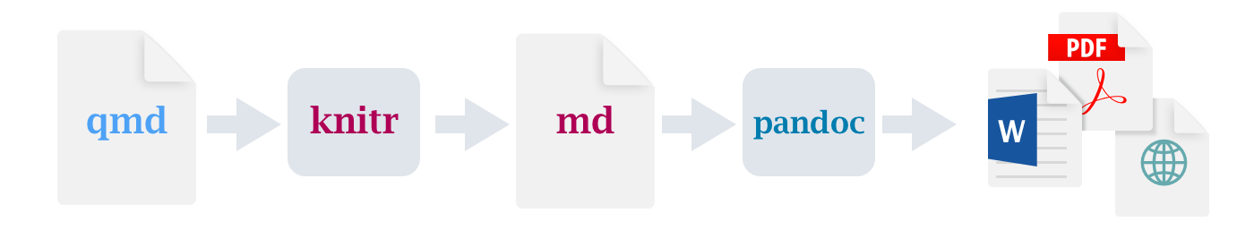
R Markdown, Quarto, knitr, and Pandoc

  • R Markdown(.Rmd) and Quarto (.qmd) files are a mix of Markdown and R code
  • knitr is an R package which evaluates R code and returns the output as a Markdown file
  • Pandoc is a separate (independent) program that converts Markdown to a variety of formats
How Quarto works: qmd to knitr to md to pandoc to multiple formats including pdf, HTML and Microsoft Word

R Markdown vs. Quarto
Quarto (.qmd) is the next generation of R Markdown (.Rmd). You can still use R Markdown (it’s not going anywhere), but Quarto is much newer and more powerful.

Terminology

YAML, HTML, CSS/SCSS

  • YAML is a language for specifying metadata
    • Used for specifying document options and chunk options
  • HTML is a language for making websites
    • Can be used directly in .qmd/.Rmd files if you plan to output to HTML
    • E.g., can use <br> for a line break
  • CSS is a language for styling websites
    • Can be used to apply custom styles to documents
    • SCSS is CSS with superpowers

Some options

Document level options - YAML block

---
title: "My great analysis"
format: html
date: today
toc: true
code-fold: true
---
  • date: today to include today’s date
  • toc: true to include a table of contents
  • code-fold: true to hide code (with option to show)

Note: These are Quarto options! R Markdown has similar ones, but they may be slightly different. E.g., format: html_document in R Markdown.

Some options

Chunk level options - YAML notation

```{r}
#| fig-width: 10
#| fig-asp: 0.5
#| fig-alt: |
#|   A scatterplot in black and white showing degree of 
#|   urbanization on the x-axis and number of songs on 
#|   the y-axis with no appreciable pattern in the data.
#| fig-cap: |
#|   The relationship between urbanization and the number
#|   of songs in mountain chickadee dawn choruses.

ggplot(data = my_data, aes(x = urbanization, y = songs)) +
  geom_point()
```
  • fig-width width of figure in inches
  • fig-asp aspect of the figure (1 = square) (i.e. height = width * aspect)
  • fig-alt Accessibility Alt text for screen readers helping those who can’t see the figure (should be descriptive, not the same as a caption)
  • fig-cap Figure caption

Gives…

ggplot(data = my_data, aes(x = urbanization, y = songs)) +
  geom_point()
A scatterplot in black and white showing degree of urbanization on the x-axis and number of songs on the y-axis with no appreciable pattern in the data.

The relationship between urbanization and the number of songs in mountain chickadee dawn choruses.

Enhancing reproducibility

  • Make your publication figures in reports
  • Date your reports (my_analysis_2022-09-08.html)
  • Include info on packages used (because you’re going to cite them… right? RIGHT?)
    • devtools::session_info()
    • report::report_packages()
    • report::cite_packages()
  • Embed data directly (for smaller datasets) using DT package
DT::datatable(mtcars, extensions = 'Buttons',
              options = list(dom = 'Bfrtip', buttons = c('csv', 'excel')))

Cite the Packages!

Seriously, cite the packages 😁

Your Turn

Use the more advanced template (example.qmd) to create a reproducible report of your analysis.

Consider the options we learned

Anything you’d like to add?

Some Final Thoughts

Rendering vs. Spinning

Rendering (Render/Knit button)

.Rmd/.qmd

.md

HTML
  • Good for lots of text
  • Better option control
  • Use ```{r} and ```to define code blocks

Spinning (Knit button)

.R

.md

HTML
  • Easier to code
  • Use #' to define markdown
  • Use #+ to define chunk options
    • Use Rmarkdown option style
    • i.e., error=FALSE not error: false

Rendering vs. Spinning

Rendering (Render/Knit button)


## Setup
This is my **great** study.... I used these packages:

```{r}
library(tidyverse)
```

## Loading data
These are the datasets I used

```{r}
my_data <- read_csv("https://raw.githubusercontent.com/steffilazerte/NRI_7350/main/data/chorus.csv")
my_data
```

This is what it looks like

```{r}
#| fig-width: 6
ggplot(data = my_data, aes(x = urbanization, y = songs)) +
  geom_point()
```

Or render with:

quarto::quarto_render(
  input = "example.qmd", 
  output_file = paste0("example_", Sys.Date(), ".html"))

Spinning (Knit button)

#' ## Setup
#' This is my **great** study.... I used these packages:

library(tidyverse)

#' ## Loading data
#' These are the datasets I used

my_data <- read_csv("https://raw.githubusercontent.com/steffilazerte/NRI_7350/main/data/chorus.csv")
my_data

#' This is what it looks like

#+ fig-width = 6
ggplot(data = my_data, aes(x = urbanization, y = songs)) +
  geom_point()

Or spin/render with:

knitr::spin("example_spin.R", knit = FALSE)
quarto::quarto_render(
  input = "example_spin.Rmd",
  output_file = paste0("example_spin_", Sys.Date(), ".html"))

Relative locations

If you use nested folders in your work,
you’ll want to use the here package to ensure
all the file locations are consistent

library(here)
library(tidyverse)

my_data <- read_csv(here("Data/my_data.csv"))

A cartoon showing two paths side-by-side. On the left is a scary spooky forest, with spiderwebs and gnarled trees, with file paths written on the branches like '~/mmm/nope.csv' and 'setwd('/haha/good/luck/')', with a scared looking cute fuzzy monster running out of it. On the right is a bright, colorful path with flowers, rainbow and sunshine, with signs saying 'here!' and 'it’s all right here!' A monster facing away from us in a backpack and walking stick is looking toward the right path. Stylized text reads 'here: find your path.'

Artwork by @allison_horst

Resources

Online References

Slides created with Quarto Updated 2023-04-17