class: title-slide, nobar  ## Workshop: Dealing with Data in R # Getting started with R ## Back to Basics .footnote[Steffi LaZerte <https://steffilazerte.ca> | *Compiled: 2022-01-28*] --- class: space-list # Online workshops can be challenging - **Consider keeping your video on** .small[(if possible)] - We're here together! - Kids? Pets? Spouses? No problem - But ultimately, you need be comfortable! .small[(and you absolutely have the right to privacy at home)] - **Interrupt me!** - Generally keep yourself muted but un-mute anytime to ask questions - **Ask Questions!** - Group trouble-shooting is really valuable - If you have a problem, others may also (or may have it in the future) - **Screen-sharing** - I may ask you to share your screen with the group .small[(feel free to decline)] - For privacy, close your email etc. Or just share your RStudio window --- class: nobar background-image: url(figures/office.jpg) background-size: cover background-position: center # **This is me!** --- class: nobar   # **These are my creatures** --- class: nobar 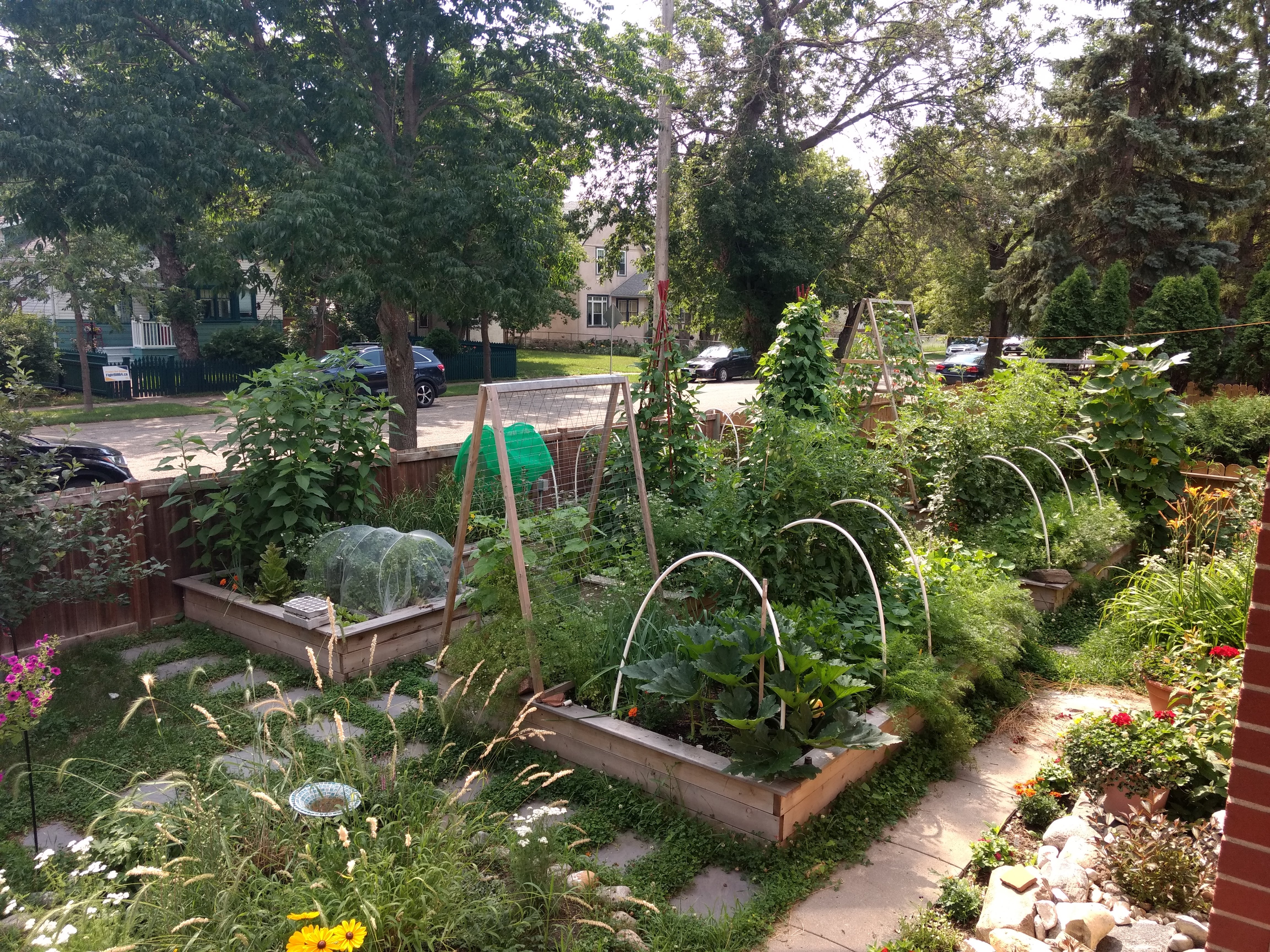 # **This is my garden** --- # **This is my work***             .footnote[.small[(* On, with, and for)]] --- background-image: url(figures/office.jpg) background-position: right 25px bottom 50px background-size: 50% # Introductions ## Dr. Steffi LaZerte - Background in Biology (Animal Behaviour) - Working with R since 2007 - Professional R programmer/consultant<br>since 2017 - Fourth year giving BU R Workshop! - [rOpenSci](https://ropensci.org) Community Assistant --- background-image: url(figures/alex.jpg) background-position: right 25px bottom 25px background-size: 40% # Introductions ## Dr. Alex Koiter ### Backup helper today - Physical Geographer - Working with R since 2010 - Assistant Professor in Geography and Environment, Brandon University --- class: space-list # What about you? - Name - Creatures? (share on camera!) - Background (Role, Area of study, etc.) - Familiarity with R or Programming - Something you're proud of! --- # About this Workshop ## Format - I will provide you tools and workflow to get started with R - We'll have hands-on, lecture, and demonstrations .spacer[] ## R is hard: But have no fear! - Don't expect to remember everything! - Copy/Paste is your friend (never apologize for using it!) - Consider this workshop a resource to return to --- # About this Workshop ## Format - I will provide you tools and workflow to get started with R - We'll have hands-on, lecture, and demonstrations .spacer[] ## R is hard: But have no fear! - **Don't expect to remember everything!** - Copy/Paste is your friend (never apologize for using it!) - Consider this workshop a resource to return to --- background-image: url(figures/impostR_en.png) background-position: center center background-size: 70% # Impost**R** Syndrome --- background-image: url(figures/impostR_en.png) background-position: right 75px top 25% background-size: 30% # Impost**R** Syndrome 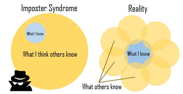 --  --- class: nobar  .footnote[Artwork by [@allison_horst](https://github.com/allisonhorst/stats-illustrations)] --- class: section # All about R --- layout: true # Why R? --- background-image: url(figures/R_hard.png) background-position: right 15% bottom 10% background-size: 70% ## R is hard --- background-image: url(figures/R_powerful2_edit.png) background-position: center bottom 40% background-size: 70% ## But R is powerful (and reproducible)! -- .footnote[(I made these slides with **R**markdown)] --- background-image: url(figures/spatial.png) background-position: center bottom 10% background-size: 40% ## R is also beautiful --- background-image: url(figures/R_free.png) background-position: center bottom 40% background-size: 70% ## R is affordable (i.e., free!) --- layout: false class: section # What is R? --- # R is Programming language > A programming **language** is a way to give instructions in order to get a computer to do something - You need to know the language (i.e., the code) - Computers don't know what you mean, only what you type (unfortunately) - Spelling, punctuation, and capitalization all matter! ## For example **R, what is 56 times 5.8?** ```r 56 * 5.8 ``` ``` ## [1] 324.8 ``` --- # Use code to tell R what to do **R, what is the average of numbers 1, 2, 3, 4?** ```r mean(c(1, 2, 3, 4)) ``` ``` ## [1] 2.5 ``` -- **R, save this value for later** ```r steffis_mean <- mean(c(1, 2, 3, 4)) ``` -- **R, multiply this value by 6** ```r steffis_mean * 6 ``` ``` ## [1] 15 ``` --- class: split-50 # Code, Output, Scripts .columnl[ ## Code - The actual commands ## Output - The result of running code or a script ## Script - A text file full of code that you want to run - You should always keep your code in a script ] -- .columnr[ ## For example: ```r mean(c(1, 2, 3, 4)) ``` ``` ## [1] 2.5 ``` ]    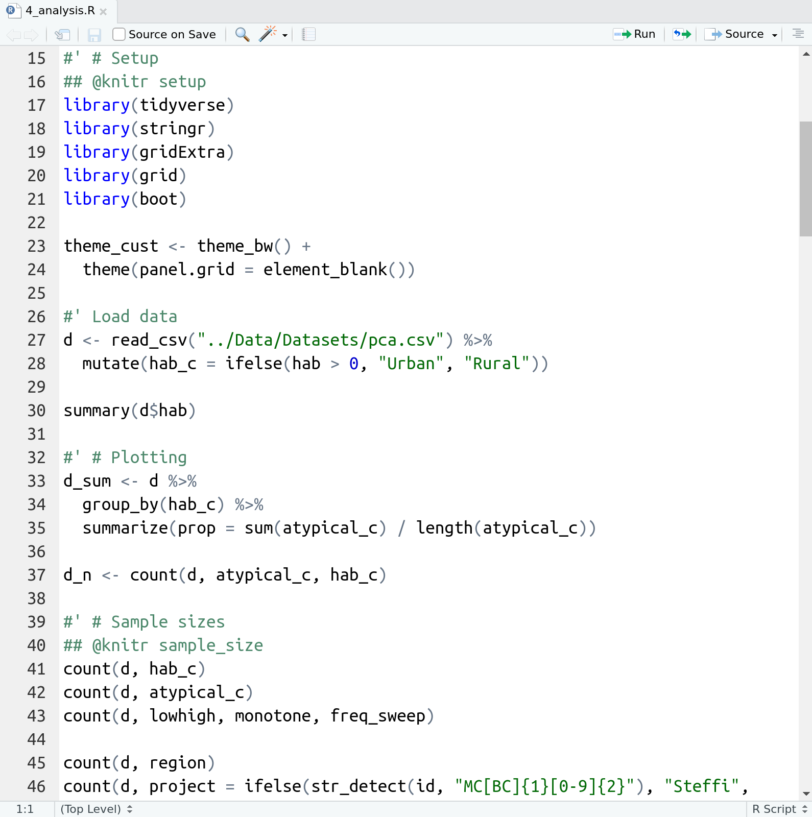 --- # RStudio vs. R   ![:spacer 175px]() - **RStudio** is not **R** - RStudio is a User Interface or IDE (integrated development environment) - (i.e., Makes coding simpler) - But sometimes tries to be **too** helpful --- # RStudio Features ## Changing Options: Tools > Global Options - General > Restore RData into workspace at startup (NO!) - General > Save workspace to on exit (NEVER!) - Code > Insert matching parens/quotes (Personal preference) ## Projects - Handles working directories - Organizes your work ## Packages - Can use the package manager to install packages - Can use the manager to load them as well, but not recommended --- class: section # Let's take a look at RStudio --- class: section # Your first *real* code! --- # First Code <code class ='r hljs remark-code'># First load the packages<br>library(tidyverse)<br>library(palmerpenguins)<br><br># Now create the figure<br>ggplot(data = penguins, aes(x = body_mass_g, y = flipper_length_mm, colour = species)) +<br> geom_point()</code> .spacer[ ] - Copy/paste or type this into the script window in RStudio - You may have to go to File > New File > R Script - Click anywhere on the first line of code - Use the 'Run' button to run this code, **or** use the short-cut `Ctrl-Enter` - Repeat until all the code has run --- layout: true # First Code --- <code class ='r hljs remark-code'># First load the packages<br>library(tidyverse)<br>library(palmerpenguins)<br><br># Now create the figure<br>ggplot(data = penguins, aes(x = body_mass_g, y = flipper_length_mm, colour = species)) +<br> geom_point()</code> ``` ## Warning: Removed 2 rows containing missing values (geom_point). ``` <img src="1 Introduction to R_files/figure-html/first_code-flaired-e3oxvgu-1.png" width="60%" style="display: block; margin: auto;" /> --- <code class ='r hljs remark-code'># First load the packages<br>library(<span style="background-color:#ffff7f">tidyverse</span>)<br>library(<span style="background-color:#ffff7f">palmerpenguins</span>)<br><br># Now create the figure<br>ggplot(data = penguins, aes(x = body_mass_g, y = flipper_length_mm, colour = species)) +<br> geom_point()</code> ``` ## Warning: Removed 2 rows containing missing values (geom_point). ``` <img src="1 Introduction to R_files/figure-html/first_code-flaired-0rxvajl-1.png" width="60%" style="display: block; margin: auto;" />  --- <code class ='r hljs remark-code'># First load the packages<br><span style="background-color:#ffff7f">library</span>(tidyverse)<br><span style="background-color:#ffff7f">library</span>(palmerpenguins)<br><br># Now create the figure<br><span style="background-color:#ffff7f">ggplot</span>(data = penguins, <span style="background-color:#ffff7f">aes</span>(x = body_mass_g, y = flipper_length_mm, colour = species)) +<br> <span style="background-color:#ffff7f">geom_point</span>()</code> ``` ## Warning: Removed 2 rows containing missing values (geom_point). ``` <img src="1 Introduction to R_files/figure-html/first_code-flaired-8eykdd5-1.png" width="60%" style="display: block; margin: auto;" /> </code>, <code>ggplot()</code><br><code>aes()</code>, and <code>geom_point()</code>) --- <code class ='r hljs remark-code'># First load the packages<br>library(tidyverse)<br>library(palmerpenguins)<br><br># Now create the figure<br>ggplot(data = penguins, aes(x = body_mass_g, y = flipper_length_mm, colour = species)) <span style="background-color:#ffff7f">+</span><br> geom_point()</code> ``` ## Warning: Removed 2 rows containing missing values (geom_point). ``` <img src="1 Introduction to R_files/figure-html/first_code-flaired-3xibawh-1.png" width="60%" style="display: block; margin: auto;" /> ) --- <code class ='r hljs remark-code'># First load the packages<br>library(tidyverse)<br>library(palmerpenguins)<br><br># Now create the figure<br>ggplot(data = penguins, aes(x = body_mass_g, y = flipper_length_mm, colour = species)) +<br> geom_point()</code> ``` ## Warning: Removed 2 rows containing missing values (geom_point). ``` <img src="1 Introduction to R_files/figure-html/first_code-flaired-e7bd7wz-1.png" width="60%" style="display: block; margin: auto;" />  --- <code class ='r hljs remark-code'># First load the packages<br>library(tidyverse)<br>library(palmerpenguins)<br><br># Now create the figure<br>ggplot(data = penguins, aes(x = body_mass_g, y = flipper_length_mm, colour = species)) +<br> geom_point()</code> ``` ## Warning: Removed 2 rows containing missing values (geom_point). ``` <img src="1 Introduction to R_files/figure-html/first_code-flaired-s3kyin0-1.png" width="60%" style="display: block; margin: auto;" />  --- <code class ='r hljs remark-code'><span style="background-color:#ffff7f"># First load the packages</span><br>library(tidyverse)<br>library(palmerpenguins)<br><br><span style="background-color:#ffff7f"># Now create the figure</span><br>ggplot(data = penguins, aes(x = body_mass_g, y = flipper_length_mm, colour = species)) +<br> geom_point()</code> ``` ## Warning: Removed 2 rows containing missing values (geom_point). ``` <img src="1 Introduction to R_files/figure-html/first_code-flaired-0gl93kx-1.png" width="60%" style="display: block; margin: auto;" /> ) --- layout:false class: section # R Basics: Objects Objects are *things* in the environment (Check out the **Environment** pane in RStudio) --- # functions() ## Do things, Return things ### Does something but returns nothing e.g., `write_csv()` - Saves the `mtcars` data frame as a csv file ```r write_csv(mtcars, path = "mtcars.csv") ``` .spacer[ ] ### Does something and returns something e.g., `sd()` - returns the standard deviation of a vector ```r sd(c(4, 10, 21, 55)) ``` ``` ## [1] 22.78157 ``` --- class: split-50 # functions() - Functions can take **arguments** (think 'options') - `data`, `x`, `y`, `colour` ```r ggplot(data = msleep, aes(x = sleep_total, y = sleep_rem, colour = vore)) + geom_point() ``` -- ![:spacer 20px]() - Arguments defined by **name** or by **position** - With correct position, do not need to specify by name ![:spacer 10px]() .columnl[ ### By name: ```r mean(x = c(1, 5, 10)) ``` ``` ## [1] 5.333333 ``` ] .columnr[ ### By order: ```r mean(c(1, 5, 10)) ``` ``` ## [1] 5.333333 ``` ] --- class: split-40 # functions() ## Watch out for 'hidden' arguments .columnl[ ### By name: ```r mean(x = c(1, 5, 10, NA), na.rm = TRUE) ``` ``` ## [1] 5.333333 ``` ] -- .columnr[ ### By order: ```r mean(c(1, 5, 10, NA), TRUE) ``` ``` ## Error in mean.default(c(1, 5, 10, NA), TRUE): 'trim' must be numeric of length one ``` ] -- ![:spacer 130px]() .center[This error states that we've assigned the argument `trim` to a non-valid argument] .spacer[ ] .center[Where did **`trim`** come from?] --- class: split-15 # R documentation .columnl[ ```r ?mean ``` ] ??? Look up trim, do you see it? -- 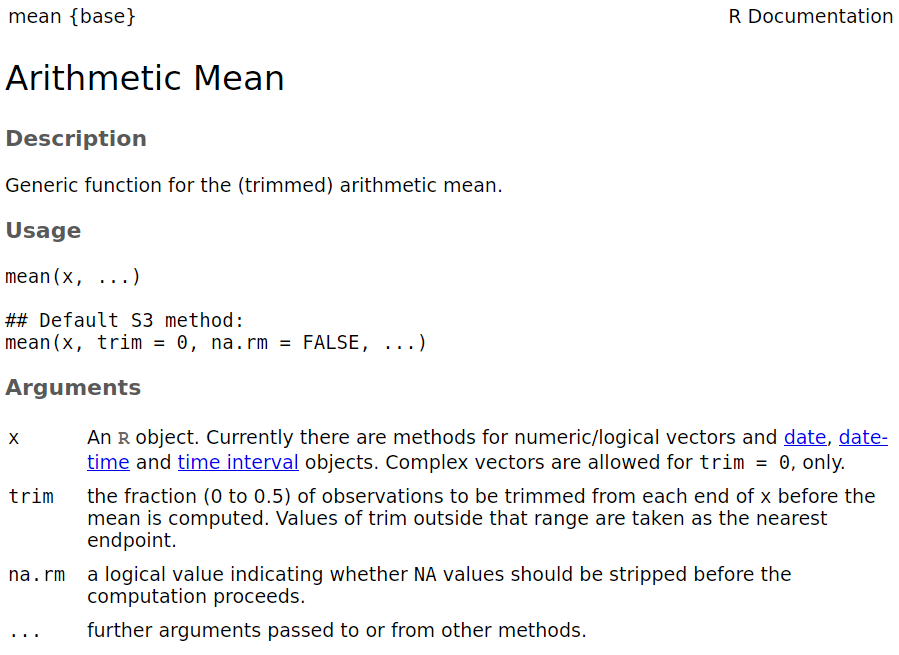 --- class: split-40 # Data Generally kept in `vectors` or `data.frames` - These are objects with names (like functions) - We can use `<-` to assign values to objects (assignment) ![:spacer 10px]() .columnl[ ## Vector (1 dimension) ```r my_letters <- c("a", "b", "c") my_letters ``` ``` ## [1] "a" "b" "c" ``` ] .columnr[ ## Data frame (2 dimensions) ```r my_data <- data.frame(x = c("s1", "s2", "s3", "s4"), y = c(101, 102, 103, 104), z = c("a", "b", "c", "d")) my_data ``` ``` ## x y z ## 1 s1 101 a ## 2 s2 102 b ## 3 s3 103 c ## 4 s4 104 d ``` ]  --- class: space # Vectors ### Use `c()` to create a vector ```r a <- c("apples", 12, "bananas") ``` ### Use `x[index]` to access part of a vector ```r a[3] # [1] "bananas" ``` ### Vectors contain one type of variable (Even if you try to make it with more) ```r class(a) # [1] "character" ``` --- # Data frames (also tibbles) ```r my_data ``` ``` ## x y z ## 1 s1 101 a ## 2 s2 102 b ## 3 s3 103 c ## 4 s4 104 d ``` - Columns have different types of variables - `x$colname` to pull columns out as vector - `x[row, col]` to access rows and columns of a data frame --- class: split-40 # Your Turn: Vectors and Data frames Try out the following code... 1. What is the output in your console? 2. How does your `environment` change (upper right panel)? ![:spacer 20px]() .columnl[ **Vectors** ```r a <- c("apples", 12, "bananas") a ``` ] .columnr[ **Data frames** ```r my_data <- data.frame(x = c("s1", "s2", "s3", "s4"), y = c(101, 102, 103, 104), z = c("a", "b", "c", "d")) my_data ``` ] --- class: split-40 # Your Turn: Vectors and Data frames Try out the following code... .columnl[ **Vectors** ```r a[2] a[2:3] # What does : do? a[c(1, 3)] # What does c() do? ``` ] .columnr[ **Data frames** ```r my_data[3, ] # Why the comma? my_data[3, 1] my_data[, 1:2] ``` ] --- exclude: TRUE class: split-40 # Your Turn: Vectors and Data frames Try out the following code... .columnl[ **Vectors** ```r a[2] ``` ``` ## [1] "12" ``` ```r a[2:3] # What does : do? ``` ``` ## [1] "12" "bananas" ``` ```r a[c(1, 3)] # What does c() do? ``` ``` ## [1] "apples" "bananas" ``` ] .columnr[ **Data frames** ```r my_data[3, ] # Why the comma? ``` ``` ## x y z ## 3 s3 103 c ``` ```r my_data[3, 1] ``` ``` ## [1] "s3" ``` ```r my_data[, 1:2] ``` ``` ## x y ## 1 s1 101 ## 2 s2 102 ## 3 s3 103 ## 4 s4 104 ``` ] --- class: section # Miscellaneous --- # R has spelling and punctuation - R cares about spelling - R is also case sensitive! (`Apple` is not the same as `apple`) - Commas are used to separate arguments in functions ## For example This is correct: ```r mean(c(5, 7, 10)) # [1] 7.333333 ``` This is **not** correct: ```r mean(c(5 7 10)) ``` ``` ## Error: <text>:1:10: unexpected numeric constant ## 1: mean(c(5 7 ## ^ ``` -- .box-r[\>80% of learning R is learning to **troubleshoot**] --- class: space # R has spelling and punctuation ### Spaces usually don't matter unless they change meanings ```r 5>=6 # [1] FALSE 5 >=6 # [1] FALSE 5 >= 6 # [1] FALSE 5 > = 6 # Error: unexpected '=' in "5 > =" ``` ### Periods don't matter either, but can be used in the same way as letters (But don't) ```r apple.oranges <- "fruit" ``` --- class: space # Assignments and Equal signs ### Use `<-` to assign values to objects ```r a <- "hello" ``` ### Use `=` to set function arguments ```r mean(x = c(4, 9, 10)) ``` ### Use `==` to determine equivalence (logical) ```r 10 == 10 # [1] TRUE 10 == 9 # [1] FALSE ``` --- layout:true # Braces/Brackets --- ## Round brackets: `()` - Identify functions (even if there are no arguments) ```r Sys.Date() # Get the Current Date ``` ``` ## [1] "2022-01-28" ``` -- - Without the `()`, R spits out information on the function: ```r Sys.Date ``` ``` ## function () ## as.Date(as.POSIXlt(Sys.time())) ## <bytecode: 0x557a57306070> ## <environment: namespace:base> ``` -- .box-br[ `()` must be associated with a **function** .small[(Well, _almost_ always)] ] --- ## Square brackets: `[]` - Extract parts of objects ```r LETTERS ``` ``` ## [1] "A" "B" "C" "D" "E" "F" "G" "H" "I" "J" "K" "L" "M" "N" "O" "P" "Q" "R" "S" ## [20] "T" "U" "V" "W" "X" "Y" "Z" ``` ```r LETTERS[1] ``` ``` ## [1] "A" ``` ```r LETTERS[26] ``` ``` ## [1] "Z" ``` -- .box-br[ `[]` have to be associated with an **object** that has dimensions .small[(Always)] ] --- layout: false # Improving code readability ### Use spaces like you would in sentences: ```r a <- mean(c(4, 10, 13)) ``` is easier to read than ```r a<-mean(c(4,10,13)) ``` ![:spacer 15px]() (But the same, coding-wise) --- # Improving code readability ### Don't be afraid to use line breaks ('Enters') to make the code more readable ![:spacer 20px]() **Hard to read** ```r a <- data.frame(exp = c("A", "B", "A", "B", "A", "B"), sub = c("A1", "A1", "A2", "A2", "A3", "A3"), res = c(10, 12, 45, 12, 12, 13)) ``` **Easier to read** ```r a <- data.frame(exp = c("A", "B", "A", "B", "A", "B"), sub = c("A1", "A1", "A2", "A2", "A3", "A3"), res = c(10, 12, 45, 12, 12, 13)) ``` ![:spacer 15px]() (But the same, coding-wise) --- class: center, nobar ### .large[Let's go!]