class: title-slide, nobar ## Workshop: Dealing with Data in R # Summarizing and Transforming ## Saving you time and sanity .footnote[Steffi LaZerte <https://steffilazerte.ca> | *Compiled: 2022-01-26*] 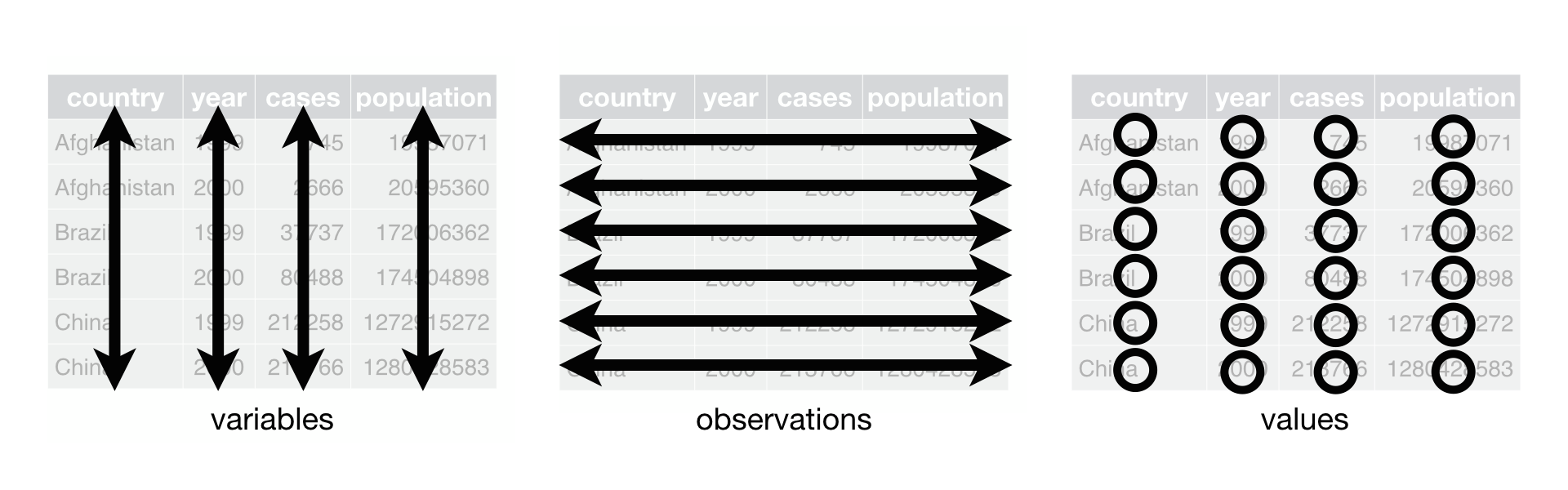 .footnote-right[Image from [R for Data Science](from http://r4ds.had.co.nz/)] --- class: section # First things first Save previous script Open New File <br>.medium[(make sure you're in the RStudio Project)] ![:spacer 10px]() Add `library(tidyverse)` to the top Save this new script .medium[consider names like `summarizing.R` or `4_summarizing_and_transforming.R`] --- class: split-50 # Types of Modifications .columnl[ ### 1. **Subset** - Subset by observations (rows) - Subset by variables (columns) - `filter()` and `select()` ![:spacer 10px]() ### 2. **Joining data sets** - `left_join()`, `right_join()`, etc. ![:spacer 10px]() ### 3. **Creating new columns** - Creating categories - Column calculations - By group - `mutate()` and `group_by()` ] .columnr[ ### 4. **Summarize existing columns** - Summarizing by group - `summarize()` and `group_by()` ![:spacer 30px]() ### 5. **Transpose** - Going between **wide** and **long** data formats - `pivot_wider()` and `pivot_longer()` - Transposing for analysis - Transposing for visualizations ] --- class: split-50 # Getting ready .columnl[ ### Check out the data: ```r library(tidyverse) size <- read_csv("data/grain_size2.csv") size ``` ] .columnr[ ### Using data sets: - [grain_size2.csv](https://steffilazerte.ca/BU-R-Workshop/data/grain_size2.csv) - [grain_meta.csv](https://steffilazerte.ca/BU-R-Workshop/data/grain_meta.csv) ] ![:spacer 65px]() ``` ## # A tibble: 114 × 9 ## plot depth coarse_sand medium_sand fine_sand coarse_silt medium_silt fine_silt clay ## <chr> <dbl> <dbl> <dbl> <dbl> <dbl> <dbl> <dbl> <dbl> ## 1 CSP01 4 13.0 17.4 19.7 14.1 11.2 8.17 16.3 ## 2 CSP01 12 10.7 16.9 19.2 14.1 11.7 9.03 18.4 ## 3 CSP01 35 12.1 17.8 16.1 10.3 9.51 7.47 26.7 ## 4 CSP01 53 17.6 18.2 14.3 9.4 9.1 8.7 22.7 ## 5 CSP01 83 21.0 18.4 14.3 9.79 8.79 7.29 20.4 ## 6 CSP01 105 19.0 18.4 14.4 10.8 9.4 8.22 19.7 ## 7 CSP08 10 11.6 17.1 20.8 16.3 9.55 6.23 18.4 ## 8 CSP08 27 15.4 16.2 17.8 14.3 10.4 6.1 19.6 ## 9 CSP08 90 14.9 15.8 18.6 15.1 11.5 7.56 16.5 ## 10 CSP02 5 8.75 8.64 8.66 12.0 18.3 15.2 28.5 ## # … with 104 more rows ``` --- class: section # Subsetting ## By rows and column --- # Subsetting: By rows ### `filter()` .small[(`tidyverse` function, specifically from `dplyr` package)] ![:spacer 20px]() .regular[ <code class ='r hljs remark-code'>filter(<strong><span style="color:#440154">data</span></strong>, <strong><span style="color:#277F8E">expression1</span></strong>, <strong><span style="color:#277F8E">expression2</span></strong>, etc.)</code> ] ![:spacer 20px]() - `tidyverse` functions always start with <strong><span style="color:#440154">data</span></strong> - <strong><span style="color:#277F8E">Column</span></strong> expressions reference actual <strong><span style="color:#277F8E">columns</span></strong> in <strong><span style="color:#440154">data</span></strong> - Here logical statments relating to <strong><span style="color:#277F8E">column</span></strong> values --- # Subsetting: By rows ## Subset by category ```r filter(size, plot %in% c("CSP11", "CSP13")) ``` .small[ ``` ## # A tibble: 9 × 9 ## plot depth coarse_sand medium_sand fine_sand coarse_silt medium_silt fine_silt clay ## <chr> <dbl> <dbl> <dbl> <dbl> <dbl> <dbl> <dbl> <dbl> ## 1 CSP13 2 22.1 17.5 18.3 11.9 7.92 6.05 16.3 ## 2 CSP13 10 12.1 14.9 18 13.1 10.4 7.92 23.6 ## 3 CSP13 25 13.7 12.7 14.3 11.7 9.67 6.31 31.6 ## 4 CSP13 60 27.1 9.74 11.1 9.69 9.79 7.82 24.8 ## 5 CSP13 140 10.4 15.3 16.0 12.4 12.4 10.2 23.5 ## 6 CSP11 20 6.67 3.94 5.52 23.7 23 14.8 22.3 ## 7 CSP11 30 5.27 4.23 6.11 23.6 23.9 15.3 21.6 ## 8 CSP11 47 4.34 4.03 6.62 24.5 25.5 13.8 21.3 ## 9 CSP11 143 5.28 4.26 7.07 22.8 28.0 12.4 20.2 ``` ] -- > Note: To save this as a separate object, don't forget assignments: ```r size_sub <- filter(size, plot %in% c("CSP11", "CSP13")) ``` --- # Subsetting: By rows ## Subset by measures ```r filter(size, depth > 140 | depth < 4) ``` ``` ## # A tibble: 9 × 9 ## plot depth coarse_sand medium_sand fine_sand coarse_silt medium_silt fine_silt clay ## <chr> <dbl> <dbl> <dbl> <dbl> <dbl> <dbl> <dbl> <dbl> ## 1 CSP13 2 22.1 17.5 18.3 11.9 7.92 6.05 16.3 ## 2 CSP19 190 3.33 4.28 14.2 42.8 21.5 9.92 4 ## 3 CSP11 143 5.28 4.26 7.07 22.8 28.0 12.4 20.2 ## 4 CSP14 3 16.1 15.0 17.5 12.2 12 9.88 17.3 ## 5 CSP15 146 13.6 12.3 12.5 12.0 18.1 10.4 21.1 ## 6 CSP20 3 5.12 5.09 17.9 25.9 14.3 11.8 19.9 ## 7 CSP20 150 22.7 12.9 12.7 17.7 14.9 7.59 11.5 ## 8 CSP21 3 14.1 11.6 11.9 14.1 15.5 10.4 22.4 ## 9 CSP22 182 17.9 13.6 13.1 13.5 12.6 8.39 20.9 ``` --- class: split-30, table-left # Tangent: Logical Operators .columnl[ ### Possible options ![:spacer 10px]() .small[ Operator | Code ---------- | ------ OR | <code>&vert;</code> AND | `&` EQUAL | `==` NOT EQUAL | `!=` NOT | `!` Greater than | `>` Less than | `<` Greater than or equal to | `>=` Less than or equal to | `<=` In | `%in%` ]] -- .columnr[ ### Single comparisons ```r 1 < 2 1 != 2 ``` ### Multiple comparisons ```r 1 == c(1, 2, 1, "apple") 1 %in% c(1, 2, 1, "apple") c(1, 2, 1, "apple") == 1 c(1, 2, 1, "apple") %in% 1 c(1, 2, 1, "apple") == 1 | c(1, 2, 1, "apple") == 2 ``` > **Your turn!** > In each case, what are you asking? Do you expect 1 or 4 values? ] --- # Subsetting: By rows ### Which values are greater than 100 OR less than 4? .small[ ```r size$depth > 140 | size$depth < 4 ``` ``` ## [1] FALSE FALSE FALSE FALSE FALSE FALSE FALSE FALSE FALSE FALSE FALSE FALSE FALSE FALSE FALSE FALSE FALSE FALSE ## [19] FALSE FALSE FALSE FALSE FALSE FALSE FALSE FALSE FALSE FALSE FALSE FALSE FALSE FALSE FALSE FALSE FALSE FALSE ## [37] TRUE FALSE FALSE FALSE FALSE FALSE FALSE FALSE FALSE FALSE FALSE FALSE FALSE FALSE FALSE FALSE FALSE FALSE ## [55] TRUE FALSE FALSE FALSE FALSE FALSE FALSE FALSE FALSE FALSE FALSE FALSE FALSE FALSE FALSE FALSE FALSE FALSE ## [73] FALSE FALSE FALSE FALSE FALSE FALSE FALSE TRUE TRUE FALSE FALSE FALSE FALSE TRUE FALSE FALSE FALSE TRUE ## [91] FALSE FALSE FALSE TRUE TRUE FALSE FALSE FALSE FALSE FALSE FALSE FALSE TRUE FALSE FALSE FALSE FALSE FALSE ## [109] FALSE FALSE FALSE FALSE FALSE FALSE ``` ] ### Return only rows with `TRUE` ```r filter(size, depth > 140 | depth < 4) ``` --- # Subsetting: By rows ## Subset by combination ```r filter(size, * depth > 100, plot %in% c("CSP11", "CSP13")) ``` ``` ## # A tibble: 2 × 9 ## plot depth coarse_sand medium_sand fine_sand coarse_silt medium_silt fine_silt clay ## <chr> <dbl> <dbl> <dbl> <dbl> <dbl> <dbl> <dbl> <dbl> ## 1 CSP13 140 10.4 15.3 16.0 12.4 12.4 10.2 23.5 ## 2 CSP11 143 5.28 4.26 7.07 22.8 28.0 12.4 20.2 ``` -- ### Equivalent (&) ```r filter(size, * depth > 100 & plot %in% c("CSP11", "CSP13")) ```  --- # Subsetting: By columns ### `select()` .small[(`tidyverse` function, specifically from `dplyr` package)] ![:spacer 20px]() .regular[ <code class ='r hljs remark-code'>select(<strong><span style="color:#440154">data</span></strong>, <strong><span style="color:#277F8E">selection1</span></strong>, <strong><span style="color:#277F8E">selection2</span></strong>, etc.)</code> ] ![:spacer 20px]() - `tidyverse` functions always start with <strong><span style="color:#440154">data</span></strong> - Specify <strong><span style="color:#277F8E">columns</span></strong> to keep or remove - <strong><span style="color:#277F8E">Column</span></strong> selections reference actual <strong><span style="color:#277F8E">columns</span></strong> in <strong><span style="color:#440154">data</span></strong> --- class: split-55 # Subsetting: By columns .columnl[ ## Subset by variable (i.e., column) .medium[ ```r select(size, coarse_sand, medium_sand, fine_sand) ``` ``` ## # A tibble: 114 × 3 ## coarse_sand medium_sand fine_sand ## <dbl> <dbl> <dbl> ## 1 13.0 17.4 19.7 ## 2 10.7 16.9 19.2 ## 3 12.1 17.8 16.1 ## 4 17.6 18.2 14.3 ## # … with 110 more rows ``` ]] -- .columnr[ ## Using helper functions .medium[ ```r select(size, ends_with("sand")) ``` ``` ## # A tibble: 114 × 3 ## coarse_sand medium_sand fine_sand ## <dbl> <dbl> <dbl> ## 1 13.0 17.4 19.7 ## 2 10.7 16.9 19.2 ## 3 12.1 17.8 16.1 ## 4 17.6 18.2 14.3 ## # … with 110 more rows ``` ]] -- .small[.compact[.center[ **Some other helper functions (`?select_helpers`):** ] Function | Usage --------------- | --------- `starts_with()` | `starts_with("fine")` `contains()` | `contains("sand")` `everything()` | Useful for rearranging `matches()` | Uses regular expressions ]] --- class: split-50 # Subsetting: By columns ## Put it all together .columnl[ ### To explore the data ```r size %>% filter(depth > 100, plot %in% c("CSP13", "CSP25")) %>% select(plot, depth, ends_with("sand")) ``` ``` ## # A tibble: 2 × 5 ## plot depth coarse_sand medium_sand fine_sand ## <chr> <dbl> <dbl> <dbl> <dbl> ## 1 CSP13 140 10.4 15.3 16.0 ## 2 CSP25 130 18.6 21.3 13.8 ``` ] -- .columnr[ ### To save as a separate object ```r *size_sub_sand <- size %>% filter(depth > 100, plot %in% c("CSP13", "CSP25")) %>% select(plot, depth, ends_with("sand")) ``` ] --- # Your turn: Subsetting - Subset the data to variables **plot**, **depth** and all measures of **sand** - Keep only values where there is **<u>at least</u> 30% clay** ```r size <- read_csv("data/grain_size2.csv") %>% * filter(???) %>% * select(???) ``` > All particle values are percentages (depth is cm)  --- exclude: FALSE # Your turn: Subsetting - Subset the data to variables **plot**, **depth** and all measures of **sand** - Keep only values where there is **<u>at least</u> 30% clay** ```r size <- read_csv("data/grain_size2.csv") %>% filter(clay >= 30) %>% select(plot, depth, ends_with("sand")) head(size) ``` ``` ## # A tibble: 2 × 5 ## plot depth coarse_sand medium_sand fine_sand ## <chr> <dbl> <dbl> <dbl> <dbl> ## 1 CSP02 36 8.15 9.24 8.55 ## 2 CSP13 25 13.7 12.7 14.3 ``` --- exclude: FALSE # Your turn: Subsetting - Subset the data to variables **plot**, **depth** and all measures of **sand** - Keep only values where there is **<u>at least</u> 30% clay** ```r size <- read_csv("data/grain_size2.csv") %>% filter(clay >= 30) %>% select(plot, depth, ends_with("sand")) head(size) ``` **Select equivalents:** - `select(plot, depth, ends_with("sand"))` - `select(plot, depth, contains("sand"))` - `select(plot, depth, coarse_sand, medium_sand, fine_sand)` - `select(-coarse_silt, -medium_silt, -fine_silt, -clay)` --- exclude: FALSE # Your turn: Subsetting (Extra Challenge) **What happens if you `select()` before you `filter()`?** ![:spacer 10px]() ```r size <- read_csv("data/grain_size2.csv") %>% select(plot, depth, ends_with("sand")) %>% filter(clay >= 30) ``` ``` ## Error: Problem with `filter()` input `..1`. ## ℹ Input `..1` is `clay >= 30`. ## x object 'clay' not found ``` ![:spacer 10px]() - Lines are sequential - First `select()` removes column `clay` - Then `filter()` cannot find `clay` - .medium[(`object 'clay' not found`)] --- class: section # Joining/Merging --- class: split-45 # Joining data sets .columnl[ ### Measurements <div id="acohkpckkr" style="overflow-x:auto;overflow-y:auto;width:auto;height:auto;"> <style>html { font-family: -apple-system, BlinkMacSystemFont, 'Segoe UI', Roboto, Oxygen, Ubuntu, Cantarell, 'Helvetica Neue', 'Fira Sans', 'Droid Sans', Arial, sans-serif; } #acohkpckkr .gt_table { display: table; border-collapse: collapse; margin-left: auto; margin-right: auto; color: #333333; font-size: 16px; font-weight: normal; font-style: normal; background-color: #FFFFFF; width: auto; border-top-style: solid; border-top-width: 2px; border-top-color: #A8A8A8; border-right-style: none; border-right-width: 2px; border-right-color: #D3D3D3; border-bottom-style: solid; border-bottom-width: 2px; border-bottom-color: #A8A8A8; border-left-style: none; border-left-width: 2px; border-left-color: #D3D3D3; } #acohkpckkr .gt_heading { background-color: #FFFFFF; text-align: center; border-bottom-color: #FFFFFF; border-left-style: none; border-left-width: 1px; border-left-color: #D3D3D3; border-right-style: none; border-right-width: 1px; border-right-color: #D3D3D3; } #acohkpckkr .gt_title { color: #333333; font-size: 125%; font-weight: initial; padding-top: 4px; padding-bottom: 4px; border-bottom-color: #FFFFFF; border-bottom-width: 0; } #acohkpckkr .gt_subtitle { color: #333333; font-size: 85%; font-weight: initial; padding-top: 0; padding-bottom: 6px; border-top-color: #FFFFFF; border-top-width: 0; } #acohkpckkr .gt_bottom_border { border-bottom-style: solid; border-bottom-width: 2px; border-bottom-color: #D3D3D3; } #acohkpckkr .gt_col_headings { border-top-style: solid; border-top-width: 2px; border-top-color: #D3D3D3; border-bottom-style: solid; border-bottom-width: 2px; border-bottom-color: #D3D3D3; border-left-style: none; border-left-width: 1px; border-left-color: #D3D3D3; border-right-style: none; border-right-width: 1px; border-right-color: #D3D3D3; } #acohkpckkr .gt_col_heading { color: #333333; background-color: #FFFFFF; font-size: 100%; font-weight: normal; text-transform: inherit; border-left-style: none; border-left-width: 1px; border-left-color: #D3D3D3; border-right-style: none; border-right-width: 1px; border-right-color: #D3D3D3; vertical-align: bottom; padding-top: 5px; padding-bottom: 6px; padding-left: 5px; padding-right: 5px; overflow-x: hidden; } #acohkpckkr .gt_column_spanner_outer { color: #333333; background-color: #FFFFFF; font-size: 100%; font-weight: normal; text-transform: inherit; padding-top: 0; padding-bottom: 0; padding-left: 4px; padding-right: 4px; } #acohkpckkr .gt_column_spanner_outer:first-child { padding-left: 0; } #acohkpckkr .gt_column_spanner_outer:last-child { padding-right: 0; } #acohkpckkr .gt_column_spanner { border-bottom-style: solid; border-bottom-width: 2px; border-bottom-color: #D3D3D3; vertical-align: bottom; padding-top: 5px; padding-bottom: 5px; overflow-x: hidden; display: inline-block; width: 100%; } #acohkpckkr .gt_group_heading { padding: 8px; color: #333333; background-color: #FFFFFF; font-size: 100%; font-weight: initial; text-transform: inherit; border-top-style: solid; border-top-width: 2px; border-top-color: #D3D3D3; border-bottom-style: solid; border-bottom-width: 2px; border-bottom-color: #D3D3D3; border-left-style: none; border-left-width: 1px; border-left-color: #D3D3D3; border-right-style: none; border-right-width: 1px; border-right-color: #D3D3D3; vertical-align: middle; } #acohkpckkr .gt_empty_group_heading { padding: 0.5px; color: #333333; background-color: #FFFFFF; font-size: 100%; font-weight: initial; border-top-style: solid; border-top-width: 2px; border-top-color: #D3D3D3; border-bottom-style: solid; border-bottom-width: 2px; border-bottom-color: #D3D3D3; vertical-align: middle; } #acohkpckkr .gt_from_md > :first-child { margin-top: 0; } #acohkpckkr .gt_from_md > :last-child { margin-bottom: 0; } #acohkpckkr .gt_row { padding-top: 8px; padding-bottom: 8px; padding-left: 5px; padding-right: 5px; margin: 10px; border-top-style: solid; border-top-width: 1px; border-top-color: #D3D3D3; border-left-style: none; border-left-width: 1px; border-left-color: #D3D3D3; border-right-style: none; border-right-width: 1px; border-right-color: #D3D3D3; vertical-align: middle; overflow-x: hidden; } #acohkpckkr .gt_stub { color: #333333; background-color: #FFFFFF; font-size: 100%; font-weight: initial; text-transform: inherit; border-right-style: solid; border-right-width: 2px; border-right-color: #D3D3D3; padding-left: 12px; } #acohkpckkr .gt_summary_row { color: #333333; background-color: #FFFFFF; text-transform: inherit; padding-top: 8px; padding-bottom: 8px; padding-left: 5px; padding-right: 5px; } #acohkpckkr .gt_first_summary_row { padding-top: 8px; padding-bottom: 8px; padding-left: 5px; padding-right: 5px; border-top-style: solid; border-top-width: 2px; border-top-color: #D3D3D3; } #acohkpckkr .gt_grand_summary_row { color: #333333; background-color: #FFFFFF; text-transform: inherit; padding-top: 8px; padding-bottom: 8px; padding-left: 5px; padding-right: 5px; } #acohkpckkr .gt_first_grand_summary_row { padding-top: 8px; padding-bottom: 8px; padding-left: 5px; padding-right: 5px; border-top-style: double; border-top-width: 6px; border-top-color: #D3D3D3; } #acohkpckkr .gt_striped { background-color: rgba(128, 128, 128, 0.05); } #acohkpckkr .gt_table_body { border-top-style: solid; border-top-width: 2px; border-top-color: #D3D3D3; border-bottom-style: solid; border-bottom-width: 2px; border-bottom-color: #D3D3D3; } #acohkpckkr .gt_footnotes { color: #333333; background-color: #FFFFFF; border-bottom-style: none; border-bottom-width: 2px; border-bottom-color: #D3D3D3; border-left-style: none; border-left-width: 2px; border-left-color: #D3D3D3; border-right-style: none; border-right-width: 2px; border-right-color: #D3D3D3; } #acohkpckkr .gt_footnote { margin: 0px; font-size: 90%; padding: 4px; } #acohkpckkr .gt_sourcenotes { color: #333333; background-color: #FFFFFF; border-bottom-style: none; border-bottom-width: 2px; border-bottom-color: #D3D3D3; border-left-style: none; border-left-width: 2px; border-left-color: #D3D3D3; border-right-style: none; border-right-width: 2px; border-right-color: #D3D3D3; } #acohkpckkr .gt_sourcenote { font-size: 90%; padding: 4px; } #acohkpckkr .gt_left { text-align: left; } #acohkpckkr .gt_center { text-align: center; } #acohkpckkr .gt_right { text-align: right; font-variant-numeric: tabular-nums; } #acohkpckkr .gt_font_normal { font-weight: normal; } #acohkpckkr .gt_font_bold { font-weight: bold; } #acohkpckkr .gt_font_italic { font-style: italic; } #acohkpckkr .gt_super { font-size: 65%; } #acohkpckkr .gt_footnote_marks { font-style: italic; font-weight: normal; font-size: 65%; } </style> <table class="gt_table" style="table-layout: fixed;; width: 0px"> <colgroup> <col style="width:120px;"/> <col style="width:120px;"/> <col style="width:120px;"/> </colgroup> <thead class="gt_col_headings"> <tr> <th class="gt_col_heading gt_columns_bottom_border gt_center" rowspan="1" colspan="1">Plot</th> <th class="gt_col_heading gt_columns_bottom_border gt_center" rowspan="1" colspan="1">Date</th> <th class="gt_col_heading gt_columns_bottom_border gt_center" rowspan="1" colspan="1">n_birds</th> </tr> </thead> <tbody class="gt_table_body"> <tr><td class="gt_row gt_center" style="background-color: #C2FFA1; color: #000000;">A</td> <td class="gt_row gt_center" style="background-color: #FFF4A1; color: #000000;">2022-01-26</td> <td class="gt_row gt_center" style="background-color: #FFF4A1; color: #000000;">1</td></tr> <tr><td class="gt_row gt_center" style="background-color: #C2FFA1; color: #000000;">A</td> <td class="gt_row gt_center" style="background-color: #FFF4A1; color: #000000;">2022-02-19</td> <td class="gt_row gt_center" style="background-color: #FFF4A1; color: #000000;">11</td></tr> <tr><td class="gt_row gt_center" style="background-color: #C2FFA1; color: #000000;">A</td> <td class="gt_row gt_center" style="background-color: #FFF4A1; color: #000000;">2022-03-15</td> <td class="gt_row gt_center" style="background-color: #FFF4A1; color: #000000;">2</td></tr> <tr><td class="gt_row gt_center" style="background-color: #C2FFA1; color: #000000;">B</td> <td class="gt_row gt_center" style="background-color: #FFF4A1; color: #000000;">2022-04-08</td> <td class="gt_row gt_center" style="background-color: #FFF4A1; color: #000000;">4</td></tr> <tr><td class="gt_row gt_center" style="background-color: #C2FFA1; color: #000000;">B</td> <td class="gt_row gt_center" style="background-color: #FFF4A1; color: #000000;">2022-05-02</td> <td class="gt_row gt_center" style="background-color: #FFF4A1; color: #000000;">10</td></tr> <tr><td class="gt_row gt_center" style="background-color: #C2FFA1; color: #000000;">B</td> <td class="gt_row gt_center" style="background-color: #FFF4A1; color: #000000;">2022-05-26</td> <td class="gt_row gt_center" style="background-color: #FFF4A1; color: #000000;">21</td></tr> </tbody> </table> </div> ### Metadata <div id="surlqadymd" style="overflow-x:auto;overflow-y:auto;width:auto;height:auto;"> <style>html { font-family: -apple-system, BlinkMacSystemFont, 'Segoe UI', Roboto, Oxygen, Ubuntu, Cantarell, 'Helvetica Neue', 'Fira Sans', 'Droid Sans', Arial, sans-serif; } #surlqadymd .gt_table { display: table; border-collapse: collapse; margin-left: auto; margin-right: auto; color: #333333; font-size: 16px; font-weight: normal; font-style: normal; background-color: #FFFFFF; width: auto; border-top-style: solid; border-top-width: 2px; border-top-color: #A8A8A8; border-right-style: none; border-right-width: 2px; border-right-color: #D3D3D3; border-bottom-style: solid; border-bottom-width: 2px; border-bottom-color: #A8A8A8; border-left-style: none; border-left-width: 2px; border-left-color: #D3D3D3; } #surlqadymd .gt_heading { background-color: #FFFFFF; text-align: center; border-bottom-color: #FFFFFF; border-left-style: none; border-left-width: 1px; border-left-color: #D3D3D3; border-right-style: none; border-right-width: 1px; border-right-color: #D3D3D3; } #surlqadymd .gt_title { color: #333333; font-size: 125%; font-weight: initial; padding-top: 4px; padding-bottom: 4px; border-bottom-color: #FFFFFF; border-bottom-width: 0; } #surlqadymd .gt_subtitle { color: #333333; font-size: 85%; font-weight: initial; padding-top: 0; padding-bottom: 6px; border-top-color: #FFFFFF; border-top-width: 0; } #surlqadymd .gt_bottom_border { border-bottom-style: solid; border-bottom-width: 2px; border-bottom-color: #D3D3D3; } #surlqadymd .gt_col_headings { border-top-style: solid; border-top-width: 2px; border-top-color: #D3D3D3; border-bottom-style: solid; border-bottom-width: 2px; border-bottom-color: #D3D3D3; border-left-style: none; border-left-width: 1px; border-left-color: #D3D3D3; border-right-style: none; border-right-width: 1px; border-right-color: #D3D3D3; } #surlqadymd .gt_col_heading { color: #333333; background-color: #FFFFFF; font-size: 100%; font-weight: normal; text-transform: inherit; border-left-style: none; border-left-width: 1px; border-left-color: #D3D3D3; border-right-style: none; border-right-width: 1px; border-right-color: #D3D3D3; vertical-align: bottom; padding-top: 5px; padding-bottom: 6px; padding-left: 5px; padding-right: 5px; overflow-x: hidden; } #surlqadymd .gt_column_spanner_outer { color: #333333; background-color: #FFFFFF; font-size: 100%; font-weight: normal; text-transform: inherit; padding-top: 0; padding-bottom: 0; padding-left: 4px; padding-right: 4px; } #surlqadymd .gt_column_spanner_outer:first-child { padding-left: 0; } #surlqadymd .gt_column_spanner_outer:last-child { padding-right: 0; } #surlqadymd .gt_column_spanner { border-bottom-style: solid; border-bottom-width: 2px; border-bottom-color: #D3D3D3; vertical-align: bottom; padding-top: 5px; padding-bottom: 5px; overflow-x: hidden; display: inline-block; width: 100%; } #surlqadymd .gt_group_heading { padding: 8px; color: #333333; background-color: #FFFFFF; font-size: 100%; font-weight: initial; text-transform: inherit; border-top-style: solid; border-top-width: 2px; border-top-color: #D3D3D3; border-bottom-style: solid; border-bottom-width: 2px; border-bottom-color: #D3D3D3; border-left-style: none; border-left-width: 1px; border-left-color: #D3D3D3; border-right-style: none; border-right-width: 1px; border-right-color: #D3D3D3; vertical-align: middle; } #surlqadymd .gt_empty_group_heading { padding: 0.5px; color: #333333; background-color: #FFFFFF; font-size: 100%; font-weight: initial; border-top-style: solid; border-top-width: 2px; border-top-color: #D3D3D3; border-bottom-style: solid; border-bottom-width: 2px; border-bottom-color: #D3D3D3; vertical-align: middle; } #surlqadymd .gt_from_md > :first-child { margin-top: 0; } #surlqadymd .gt_from_md > :last-child { margin-bottom: 0; } #surlqadymd .gt_row { padding-top: 8px; padding-bottom: 8px; padding-left: 5px; padding-right: 5px; margin: 10px; border-top-style: solid; border-top-width: 1px; border-top-color: #D3D3D3; border-left-style: none; border-left-width: 1px; border-left-color: #D3D3D3; border-right-style: none; border-right-width: 1px; border-right-color: #D3D3D3; vertical-align: middle; overflow-x: hidden; } #surlqadymd .gt_stub { color: #333333; background-color: #FFFFFF; font-size: 100%; font-weight: initial; text-transform: inherit; border-right-style: solid; border-right-width: 2px; border-right-color: #D3D3D3; padding-left: 12px; } #surlqadymd .gt_summary_row { color: #333333; background-color: #FFFFFF; text-transform: inherit; padding-top: 8px; padding-bottom: 8px; padding-left: 5px; padding-right: 5px; } #surlqadymd .gt_first_summary_row { padding-top: 8px; padding-bottom: 8px; padding-left: 5px; padding-right: 5px; border-top-style: solid; border-top-width: 2px; border-top-color: #D3D3D3; } #surlqadymd .gt_grand_summary_row { color: #333333; background-color: #FFFFFF; text-transform: inherit; padding-top: 8px; padding-bottom: 8px; padding-left: 5px; padding-right: 5px; } #surlqadymd .gt_first_grand_summary_row { padding-top: 8px; padding-bottom: 8px; padding-left: 5px; padding-right: 5px; border-top-style: double; border-top-width: 6px; border-top-color: #D3D3D3; } #surlqadymd .gt_striped { background-color: rgba(128, 128, 128, 0.05); } #surlqadymd .gt_table_body { border-top-style: solid; border-top-width: 2px; border-top-color: #D3D3D3; border-bottom-style: solid; border-bottom-width: 2px; border-bottom-color: #D3D3D3; } #surlqadymd .gt_footnotes { color: #333333; background-color: #FFFFFF; border-bottom-style: none; border-bottom-width: 2px; border-bottom-color: #D3D3D3; border-left-style: none; border-left-width: 2px; border-left-color: #D3D3D3; border-right-style: none; border-right-width: 2px; border-right-color: #D3D3D3; } #surlqadymd .gt_footnote { margin: 0px; font-size: 90%; padding: 4px; } #surlqadymd .gt_sourcenotes { color: #333333; background-color: #FFFFFF; border-bottom-style: none; border-bottom-width: 2px; border-bottom-color: #D3D3D3; border-left-style: none; border-left-width: 2px; border-left-color: #D3D3D3; border-right-style: none; border-right-width: 2px; border-right-color: #D3D3D3; } #surlqadymd .gt_sourcenote { font-size: 90%; padding: 4px; } #surlqadymd .gt_left { text-align: left; } #surlqadymd .gt_center { text-align: center; } #surlqadymd .gt_right { text-align: right; font-variant-numeric: tabular-nums; } #surlqadymd .gt_font_normal { font-weight: normal; } #surlqadymd .gt_font_bold { font-weight: bold; } #surlqadymd .gt_font_italic { font-style: italic; } #surlqadymd .gt_super { font-size: 65%; } #surlqadymd .gt_footnote_marks { font-style: italic; font-weight: normal; font-size: 65%; } </style> <table class="gt_table" style="table-layout: fixed;; width: 0px"> <colgroup> <col style="width:150px;"/> <col style="width:150px;"/> </colgroup> <thead class="gt_col_headings"> <tr> <th class="gt_col_heading gt_columns_bottom_border gt_center" rowspan="1" colspan="1">Plot</th> <th class="gt_col_heading gt_columns_bottom_border gt_center" rowspan="1" colspan="1">Vegetation Density</th> </tr> </thead> <tbody class="gt_table_body"> <tr><td class="gt_row gt_center" style="background-color: #C2FFA1; color: #000000;">A</td> <td class="gt_row gt_center" style="background-color: #D1A1FF; color: #000000;">50</td></tr> <tr><td class="gt_row gt_center" style="background-color: #C2FFA1; color: #000000;">B</td> <td class="gt_row gt_center" style="background-color: #D1A1FF; color: #000000;">76</td></tr> </tbody> </table> </div> ] -- .columnr[ ### Joining them together ![:spacer 10px]() .center[Metadata is duplicated to line up with measurements] ![:spacer 10px]() <div id="pazaiasbzf" style="overflow-x:auto;overflow-y:auto;width:auto;height:auto;"> <style>html { font-family: -apple-system, BlinkMacSystemFont, 'Segoe UI', Roboto, Oxygen, Ubuntu, Cantarell, 'Helvetica Neue', 'Fira Sans', 'Droid Sans', Arial, sans-serif; } #pazaiasbzf .gt_table { display: table; border-collapse: collapse; margin-left: auto; margin-right: auto; color: #333333; font-size: 16px; font-weight: normal; font-style: normal; background-color: #FFFFFF; width: auto; border-top-style: solid; border-top-width: 2px; border-top-color: #A8A8A8; border-right-style: none; border-right-width: 2px; border-right-color: #D3D3D3; border-bottom-style: solid; border-bottom-width: 2px; border-bottom-color: #A8A8A8; border-left-style: none; border-left-width: 2px; border-left-color: #D3D3D3; } #pazaiasbzf .gt_heading { background-color: #FFFFFF; text-align: center; border-bottom-color: #FFFFFF; border-left-style: none; border-left-width: 1px; border-left-color: #D3D3D3; border-right-style: none; border-right-width: 1px; border-right-color: #D3D3D3; } #pazaiasbzf .gt_title { color: #333333; font-size: 125%; font-weight: initial; padding-top: 4px; padding-bottom: 4px; border-bottom-color: #FFFFFF; border-bottom-width: 0; } #pazaiasbzf .gt_subtitle { color: #333333; font-size: 85%; font-weight: initial; padding-top: 0; padding-bottom: 6px; border-top-color: #FFFFFF; border-top-width: 0; } #pazaiasbzf .gt_bottom_border { border-bottom-style: solid; border-bottom-width: 2px; border-bottom-color: #D3D3D3; } #pazaiasbzf .gt_col_headings { border-top-style: solid; border-top-width: 2px; border-top-color: #D3D3D3; border-bottom-style: solid; border-bottom-width: 2px; border-bottom-color: #D3D3D3; border-left-style: none; border-left-width: 1px; border-left-color: #D3D3D3; border-right-style: none; border-right-width: 1px; border-right-color: #D3D3D3; } #pazaiasbzf .gt_col_heading { color: #333333; background-color: #FFFFFF; font-size: 100%; font-weight: normal; text-transform: inherit; border-left-style: none; border-left-width: 1px; border-left-color: #D3D3D3; border-right-style: none; border-right-width: 1px; border-right-color: #D3D3D3; vertical-align: bottom; padding-top: 5px; padding-bottom: 6px; padding-left: 5px; padding-right: 5px; overflow-x: hidden; } #pazaiasbzf .gt_column_spanner_outer { color: #333333; background-color: #FFFFFF; font-size: 100%; font-weight: normal; text-transform: inherit; padding-top: 0; padding-bottom: 0; padding-left: 4px; padding-right: 4px; } #pazaiasbzf .gt_column_spanner_outer:first-child { padding-left: 0; } #pazaiasbzf .gt_column_spanner_outer:last-child { padding-right: 0; } #pazaiasbzf .gt_column_spanner { border-bottom-style: solid; border-bottom-width: 2px; border-bottom-color: #D3D3D3; vertical-align: bottom; padding-top: 5px; padding-bottom: 5px; overflow-x: hidden; display: inline-block; width: 100%; } #pazaiasbzf .gt_group_heading { padding: 8px; color: #333333; background-color: #FFFFFF; font-size: 100%; font-weight: initial; text-transform: inherit; border-top-style: solid; border-top-width: 2px; border-top-color: #D3D3D3; border-bottom-style: solid; border-bottom-width: 2px; border-bottom-color: #D3D3D3; border-left-style: none; border-left-width: 1px; border-left-color: #D3D3D3; border-right-style: none; border-right-width: 1px; border-right-color: #D3D3D3; vertical-align: middle; } #pazaiasbzf .gt_empty_group_heading { padding: 0.5px; color: #333333; background-color: #FFFFFF; font-size: 100%; font-weight: initial; border-top-style: solid; border-top-width: 2px; border-top-color: #D3D3D3; border-bottom-style: solid; border-bottom-width: 2px; border-bottom-color: #D3D3D3; vertical-align: middle; } #pazaiasbzf .gt_from_md > :first-child { margin-top: 0; } #pazaiasbzf .gt_from_md > :last-child { margin-bottom: 0; } #pazaiasbzf .gt_row { padding-top: 8px; padding-bottom: 8px; padding-left: 5px; padding-right: 5px; margin: 10px; border-top-style: solid; border-top-width: 1px; border-top-color: #D3D3D3; border-left-style: none; border-left-width: 1px; border-left-color: #D3D3D3; border-right-style: none; border-right-width: 1px; border-right-color: #D3D3D3; vertical-align: middle; overflow-x: hidden; } #pazaiasbzf .gt_stub { color: #333333; background-color: #FFFFFF; font-size: 100%; font-weight: initial; text-transform: inherit; border-right-style: solid; border-right-width: 2px; border-right-color: #D3D3D3; padding-left: 12px; } #pazaiasbzf .gt_summary_row { color: #333333; background-color: #FFFFFF; text-transform: inherit; padding-top: 8px; padding-bottom: 8px; padding-left: 5px; padding-right: 5px; } #pazaiasbzf .gt_first_summary_row { padding-top: 8px; padding-bottom: 8px; padding-left: 5px; padding-right: 5px; border-top-style: solid; border-top-width: 2px; border-top-color: #D3D3D3; } #pazaiasbzf .gt_grand_summary_row { color: #333333; background-color: #FFFFFF; text-transform: inherit; padding-top: 8px; padding-bottom: 8px; padding-left: 5px; padding-right: 5px; } #pazaiasbzf .gt_first_grand_summary_row { padding-top: 8px; padding-bottom: 8px; padding-left: 5px; padding-right: 5px; border-top-style: double; border-top-width: 6px; border-top-color: #D3D3D3; } #pazaiasbzf .gt_striped { background-color: rgba(128, 128, 128, 0.05); } #pazaiasbzf .gt_table_body { border-top-style: solid; border-top-width: 2px; border-top-color: #D3D3D3; border-bottom-style: solid; border-bottom-width: 2px; border-bottom-color: #D3D3D3; } #pazaiasbzf .gt_footnotes { color: #333333; background-color: #FFFFFF; border-bottom-style: none; border-bottom-width: 2px; border-bottom-color: #D3D3D3; border-left-style: none; border-left-width: 2px; border-left-color: #D3D3D3; border-right-style: none; border-right-width: 2px; border-right-color: #D3D3D3; } #pazaiasbzf .gt_footnote { margin: 0px; font-size: 90%; padding: 4px; } #pazaiasbzf .gt_sourcenotes { color: #333333; background-color: #FFFFFF; border-bottom-style: none; border-bottom-width: 2px; border-bottom-color: #D3D3D3; border-left-style: none; border-left-width: 2px; border-left-color: #D3D3D3; border-right-style: none; border-right-width: 2px; border-right-color: #D3D3D3; } #pazaiasbzf .gt_sourcenote { font-size: 90%; padding: 4px; } #pazaiasbzf .gt_left { text-align: left; } #pazaiasbzf .gt_center { text-align: center; } #pazaiasbzf .gt_right { text-align: right; font-variant-numeric: tabular-nums; } #pazaiasbzf .gt_font_normal { font-weight: normal; } #pazaiasbzf .gt_font_bold { font-weight: bold; } #pazaiasbzf .gt_font_italic { font-style: italic; } #pazaiasbzf .gt_super { font-size: 65%; } #pazaiasbzf .gt_footnote_marks { font-style: italic; font-weight: normal; font-size: 65%; } </style> <table class="gt_table" style="table-layout: fixed;; width: 0px"> <colgroup> <col style="width:100px;"/> <col style="width:100px;"/> <col style="width:100px;"/> <col style="width:150px;"/> </colgroup> <thead class="gt_col_headings"> <tr> <th class="gt_col_heading gt_columns_bottom_border gt_center" rowspan="1" colspan="1">Plot</th> <th class="gt_col_heading gt_columns_bottom_border gt_center" rowspan="1" colspan="1">Date</th> <th class="gt_col_heading gt_columns_bottom_border gt_center" rowspan="1" colspan="1">n_birds</th> <th class="gt_col_heading gt_columns_bottom_border gt_center" rowspan="1" colspan="1">Vegetation Density</th> </tr> </thead> <tbody class="gt_table_body"> <tr><td class="gt_row gt_center" style="background-color: #C2FFA1; color: #000000;">A</td> <td class="gt_row gt_center" style="background-color: #FFF4A1; color: #000000;">2022-01-26</td> <td class="gt_row gt_center" style="background-color: #FFF4A1; color: #000000;">1</td> <td class="gt_row gt_center" style="background-color: #D1A1FF; color: #000000;">50</td></tr> <tr><td class="gt_row gt_center" style="background-color: #C2FFA1; color: #000000;">A</td> <td class="gt_row gt_center" style="background-color: #FFF4A1; color: #000000;">2022-02-19</td> <td class="gt_row gt_center" style="background-color: #FFF4A1; color: #000000;">11</td> <td class="gt_row gt_center" style="background-color: #D1A1FF; color: #000000;">50</td></tr> <tr><td class="gt_row gt_center" style="background-color: #C2FFA1; color: #000000;">A</td> <td class="gt_row gt_center" style="background-color: #FFF4A1; color: #000000;">2022-03-15</td> <td class="gt_row gt_center" style="background-color: #FFF4A1; color: #000000;">2</td> <td class="gt_row gt_center" style="background-color: #D1A1FF; color: #000000;">50</td></tr> <tr><td class="gt_row gt_center" style="background-color: #C2FFA1; color: #000000;">B</td> <td class="gt_row gt_center" style="background-color: #FFF4A1; color: #000000;">2022-04-08</td> <td class="gt_row gt_center" style="background-color: #FFF4A1; color: #000000;">4</td> <td class="gt_row gt_center" style="background-color: #D1A1FF; color: #000000;">76</td></tr> <tr><td class="gt_row gt_center" style="background-color: #C2FFA1; color: #000000;">B</td> <td class="gt_row gt_center" style="background-color: #FFF4A1; color: #000000;">2022-05-02</td> <td class="gt_row gt_center" style="background-color: #FFF4A1; color: #000000;">10</td> <td class="gt_row gt_center" style="background-color: #D1A1FF; color: #000000;">76</td></tr> <tr><td class="gt_row gt_center" style="background-color: #C2FFA1; color: #000000;">B</td> <td class="gt_row gt_center" style="background-color: #FFF4A1; color: #000000;">2022-05-26</td> <td class="gt_row gt_center" style="background-color: #FFF4A1; color: #000000;">21</td> <td class="gt_row gt_center" style="background-color: #D1A1FF; color: #000000;">76</td></tr> </tbody> </table> </div> ] --- class: split-45 # Joining data sets .columnl[ ## Index or Metadata .small[ ```r meta <- read_csv("data/grain_meta.csv") meta ``` ``` ## # A tibble: 27 × 4 ## plot habitat technician date ## <chr> <chr> <chr> <date> ## 1 CSP01 forest Catharine 2009-05-06 ## 2 CSP02 clearcut Catharine 2009-03-15 ## 3 CSP03 forest Jason 2009-02-05 ## 4 CSP04 forest Catharine 2009-04-23 ## 5 CSP05 grassland Catharine 2009-02-17 ## 6 CSP06 clearcut Jason 2008-12-02 ## 7 CSP07 forest Jason 2009-01-10 ## 8 CSP08 grassland Catharine 2009-04-10 ## # … with 19 more rows ``` ]] .columnr[ ## Measurements .small[ ```r size <- read_csv("data/grain_size2.csv") size ``` ``` ## # A tibble: 114 × 9 ## plot depth coarse_sand medium_sand fine_sand coarse_silt ## <chr> <dbl> <dbl> <dbl> <dbl> <dbl> ## 1 CSP01 4 13.0 17.4 19.7 14.1 ## 2 CSP01 12 10.7 16.9 19.2 14.1 ## 3 CSP01 35 12.1 17.8 16.1 10.3 ## 4 CSP01 53 17.6 18.2 14.3 9.4 ## 5 CSP01 83 21.0 18.4 14.3 9.79 ## 6 CSP01 105 19.0 18.4 14.4 10.8 ## 7 CSP08 10 11.6 17.1 20.8 16.3 ## 8 CSP08 27 15.4 16.2 17.8 14.3 ## # … with 106 more rows, and 3 more variables: ## # medium_silt <dbl>, fine_silt <dbl>, clay <dbl> ``` ]] -- ![:spacer 235px]() .center[`plot` (CSP01, CSP02, etc.) identifies data in both] --- # Types of Join: Which rows to keep?  ### `left_join(x, y)` - Keep all rows in `x` - Keep rows in `y` only if they're also in `x` -- ### `right_join(x, y)` - Keep all rows in `y` - Keep rows in `x` only if they're also in `y` -- ### `inner_join(x, y)` - Keep **only** rows that exist in **both** data frames -- ### `full_join(x, y)` - Keep **all** rows that exist in **either** `x` _or_ `y` --- # Joining data sets ### `left_join()` .small[(`tidyverse` function, specifically from `dplyr` package)] .small[(applies to other joins as well)] ![:spacer 20px]() .regular[ <code class ='r hljs remark-code'>left_join(x =<strong><span style="color:#440154"> data</span></strong>, y = <strong><span style="color:magenta">data_to_join</span></strong>, by = c("<strong><span style="color:#277F8E">column1</span></strong>", "<strong><span style="color:#277F8E">column2</span></strong>"), ...)</code> ] ![:spacer 20px]() - `tidyverse` functions always start with<strong><span style="color:#440154"> data</span></strong> - Here, also reference second dataset <strong><code><span style="color:magenta">data_to_join</span></code></strong> - `by` refers <strong><span style="color:#277F8E">columns</span></strong> in<strong><span style="color:#440154"> data</span></strong> and <strong><code><span style="color:magenta">data_to_join</span></code></strong> used to join --- # Joining data sets ### Keep all measurements, only keep meta if we have a measurement ```r size <- left_join(x = size, y = meta, by = "plot") ``` -- ### OR ```r size <- right_join(x = meta, y = size, by = "plot") ``` -- .small[ ``` ## # A tibble: 6 × 12 ## plot habitat technician date depth coarse_sand medium_sand fine_sand coarse_silt medium_silt ## <chr> <chr> <chr> <date> <dbl> <dbl> <dbl> <dbl> <dbl> <dbl> ## 1 CSP01 forest Catharine 2009-05-06 4 13.0 17.4 19.7 14.1 11.2 ## 2 CSP01 forest Catharine 2009-05-06 12 10.7 16.9 19.2 14.1 11.7 ## 3 CSP01 forest Catharine 2009-05-06 35 12.1 17.8 16.1 10.3 9.51 ## 4 CSP01 forest Catharine 2009-05-06 53 17.6 18.2 14.3 9.4 9.1 ## 5 CSP01 forest Catharine 2009-05-06 83 21.0 18.4 14.3 9.79 8.79 ## 6 CSP01 forest Catharine 2009-05-06 105 19.0 18.4 14.4 10.8 9.4 ## # … with 2 more variables: fine_silt <dbl>, clay <dbl> ``` ] > For more information see R for Data Science [Chapter 13.4 Mutating joins](http://r4ds.had.co.nz/relational-data.html#mutating-joins) --- class: section # Creating columns with `mutate()` --- class: nobar  .footnote[Artwork by [@allison_horst](https://github.com/allisonhorst/stats-illustrations)] --- # Creating new columns ### `mutate()` .small[(`tidyverse` function, specifically from `dplyr` package)] ![:spacer 20px]() .regular[ <code class ='r hljs remark-code'>mutate(<strong><span style="color:#440154">data</span></strong>, <strong><span style="color:#277F8E">column1</span></strong> = <strong><span style="color:magenta">expression1</span></strong>, <strong><span style="color:#277F8E">column2</span></strong> = <strong><span style="color:magenta">expression2</span></strong>, ...)</code> ] ![:spacer 20px]() - `tidyverse` functions always start with<strong><span style="color:#440154"> data</span></strong> - Create new or modify existing <strong><span style="color:#277F8E">columns</span></strong> in the<strong><span style="color:#440154"> data</span></strong> - <strong><span style="color:#277F8E">Columns</span></strong> filled according to <strong><span style="color:magenta">expression</span></strong> --- class: split-45 # Creating new columns ```r size <- read_csv("data/grain_size2.csv") %>% mutate(total_sand = coarse_sand + medium_sand + fine_sand) ``` -- Creates new column at the end, `total_sand` ``` ## # A tibble: 6 × 10 ## plot depth coarse_sand medium_sand fine_sand coarse_silt medium_silt fine_silt clay total_sand ## <chr> <dbl> <dbl> <dbl> <dbl> <dbl> <dbl> <dbl> <dbl> <dbl> ## 1 CSP01 4 13.0 17.4 19.7 14.1 11.2 8.17 16.3 50.1 ## 2 CSP01 12 10.7 16.9 19.2 14.1 11.7 9.03 18.4 46.8 ## 3 CSP01 35 12.1 17.8 16.1 10.3 9.51 7.47 26.7 46 ## 4 CSP01 53 17.6 18.2 14.3 9.4 9.1 8.7 22.7 50.1 ## 5 CSP01 83 21.0 18.4 14.3 9.79 8.79 7.29 20.4 53.8 ## 6 CSP01 105 19.0 18.4 14.4 10.8 9.4 8.22 19.7 51.9 ``` ![:spacer 10px]() -- > **Note:** Column math is _**vectorized**_ (i.e., row by row) --- class: split-50 # Tangent: Vectorized > Vectorized functions run in parallel across vectors .columnl[ - Many functions in R are vectorized - Makes them faster, and easier ### For example, try the following: ```r a <- c(1, 2, 3) a + a a * a ``` ] -- .columnr[ - But not all functions are vectorized ![:spacer 16px]() ### For example ```r sum(a) sum(a, a) mean(a) mean(c(a, a)) ``` ] --- # Your turn: Creating new columns - Add a calculation for **total `silt`** - Check your work ```r meta <- read_csv("data/grain_meta.csv") size <- read_csv("data/grain_size2.csv") %>% left_join(meta, by = "plot") %>% mutate(total_sand = coarse_sand + medium_sand + fine_sand, * ???) ```  --- exclude: FALSE # Your turn: Creating new columns - Add a calculation for **total `silt`** - Check your work ```r meta <- read_csv("data/grain_meta.csv") size <- read_csv("data/grain_size2.csv") %>% left_join(meta, by = "plot") %>% mutate(total_sand = coarse_sand + medium_sand + fine_sand, total_silt = coarse_silt + medium_silt + fine_silt) ``` --- exclude: FALSE # Your turn: Creating new columns - Add a calculation for **total `silt`** - Check your work ```r select(size, contains("silt")) ``` ``` ## # A tibble: 114 × 4 ## coarse_silt medium_silt fine_silt total_silt ## <dbl> <dbl> <dbl> <dbl> ## 1 14.1 11.2 8.17 33.5 ## 2 14.1 11.7 9.03 34.8 ## 3 10.3 9.51 7.47 27.3 ## 4 9.4 9.1 8.7 27.2 ## 5 9.79 8.79 7.29 25.9 ## 6 10.8 9.4 8.22 28.4 ## 7 16.3 9.55 6.23 32.1 ## 8 14.3 10.4 6.1 30.8 ## 9 15.1 11.5 7.56 34.2 ## 10 12.0 18.3 15.2 45.4 ## # … with 104 more rows ``` --  --- exclude: FALSE # Your turn: Creating new columns - Add a calculation for **total `silt`** - Check your work ```r select(size, contains("silt")) %>% as.data.frame() ``` ``` ## coarse_silt medium_silt fine_silt total_silt ## 1 14.12 11.25 8.17 33.54 ## 2 14.13 11.68 9.03 34.84 ## 3 10.33 9.51 7.47 27.31 ## 4 9.40 9.10 8.70 27.20 ## 5 9.79 8.79 7.29 25.87 ## 6 10.79 9.40 8.22 28.41 ## 7 16.30 9.55 6.23 32.08 ## 8 14.27 10.44 6.10 30.81 ## 9 15.13 11.54 7.56 34.23 ## 10 11.96 18.27 15.22 45.45 ## 11 10.70 18.33 14.30 43.33 ## 12 10.68 18.96 14.45 44.09 ## 13 11.08 17.95 13.74 42.77 ## 14 11.16 16.85 12.99 41.00 ## 15 9.97 13.79 10.97 34.73 ## 16 11.17 12.88 11.17 35.22 ## 17 17.97 14.33 10.57 42.87 ## 18 17.89 15.48 10.46 43.83 ## 19 17.32 15.06 10.45 42.83 ## 20 16.42 15.71 10.20 42.33 ## 21 16.47 15.37 11.05 42.89 ## 22 13.43 10.51 6.50 30.44 ## 23 16.05 11.83 6.99 34.87 ## 24 13.14 10.83 6.62 30.59 ## 25 12.15 11.75 8.13 32.03 ## 26 13.30 10.84 7.06 31.20 ## 27 18.03 14.17 7.62 39.82 ## 28 16.70 12.24 8.71 37.65 ## 29 17.64 12.65 8.08 38.37 ## 30 17.26 13.75 8.37 39.38 ## 31 16.30 12.60 8.10 37.00 ## 32 18.04 12.33 8.68 39.05 ## 33 19.61 12.83 7.82 40.26 ## 34 16.83 12.39 7.43 36.65 ## 35 16.15 12.45 7.81 36.41 ## 36 16.24 12.18 6.94 35.36 ## 37 11.88 7.92 6.05 25.85 ## 38 13.06 10.38 7.92 31.36 ## 39 11.70 9.67 6.31 27.68 ## 40 9.69 9.79 7.82 27.30 ## 41 12.35 12.35 10.17 34.87 ## 42 10.86 10.43 6.99 28.28 ## 43 12.17 11.22 8.68 32.07 ## 44 10.04 11.66 8.10 29.80 ## 45 10.06 11.42 10.58 32.06 ## 46 35.79 21.00 12.52 69.31 ## 47 10.81 12.59 10.29 33.69 ## 48 11.13 12.16 9.58 32.87 ## 49 10.15 11.69 8.72 30.56 ## 50 32.10 19.24 13.18 64.52 ## 51 29.19 19.07 14.23 62.49 ## 52 33.82 16.65 9.89 60.36 ## 53 31.39 18.50 12.06 61.95 ## 54 10.22 11.04 8.67 29.93 ## 55 42.78 21.49 9.92 74.19 ## 56 9.75 13.08 11.97 34.80 ## 57 10.04 13.14 10.87 34.05 ## 58 9.14 12.64 9.76 31.54 ## 59 7.07 12.40 9.74 29.21 ## 60 8.18 10.59 12.37 31.14 ## 61 8.07 10.30 7.44 25.81 ## 62 12.39 17.79 11.54 41.72 ## 63 13.34 18.13 9.48 40.95 ## 64 12.71 18.75 11.87 43.33 ## 65 13.55 22.65 12.00 48.20 ## 66 23.26 15.36 10.31 48.93 ## 67 19.52 16.90 8.40 44.82 ## 68 20.89 17.62 6.01 44.52 ## 69 23.91 22.86 5.37 52.14 ## 70 24.20 20.90 4.90 50.00 ## 71 22.22 13.36 4.93 40.51 ## 72 19.68 12.90 7.65 40.23 ## 73 17.51 14.39 6.66 38.56 ## 74 16.55 19.47 9.00 45.02 ## 75 18.15 21.61 9.18 48.94 ## 76 14.59 15.55 8.10 38.24 ## 77 23.67 23.00 14.85 61.52 ## 78 23.56 23.88 15.31 62.75 ## 79 24.48 25.47 13.78 63.73 ## 80 22.75 27.98 12.41 63.14 ## 81 12.24 12.00 9.88 34.12 ## 82 11.29 12.71 7.28 31.28 ## 83 12.04 12.78 7.14 31.96 ## 84 10.24 10.88 4.27 25.39 ## 85 13.04 16.38 9.59 39.01 ## 86 11.98 18.07 10.40 40.45 ## 87 20.54 18.22 7.84 46.60 ## 88 22.32 14.05 10.75 47.12 ## 89 19.40 15.35 9.65 44.40 ## 90 25.87 14.30 11.83 52.00 ## 91 25.84 16.26 10.47 52.57 ## 92 26.42 16.54 8.49 51.45 ## 93 26.83 16.08 11.39 54.30 ## 94 17.71 14.87 7.59 40.17 ## 95 14.08 15.49 10.37 39.94 ## 96 14.84 13.92 10.24 39.00 ## 97 16.09 15.85 10.05 41.99 ## 98 18.00 16.14 10.57 44.71 ## 99 20.93 15.75 11.59 48.27 ## 100 19.42 13.57 12.69 45.68 ## 101 18.90 15.93 9.89 44.72 ## 102 16.11 14.87 10.50 41.48 ## 103 13.50 12.58 8.39 34.47 ## 104 10.69 9.83 6.37 26.89 ## 105 9.15 8.72 5.71 23.58 ## 106 7.05 8.40 3.94 19.39 ## 107 9.26 9.70 7.36 26.32 ## 108 10.20 8.00 8.00 26.20 ## 109 9.33 9.12 7.21 25.66 ## 110 6.80 8.66 8.25 23.71 ## 111 6.73 7.85 7.06 21.64 ## 112 7.21 9.21 8.61 25.03 ## 113 7.33 13.02 5.40 25.75 ## 114 9.98 9.76 6.80 26.54 ```  --- exclude: FALSE # Your turn: Creating new columns (Extra Challenge) **What happens if you add `total_sand` and `total_silt` together in the same `mutate()`?** ```r meta <- read_csv("data/grain_meta.csv") size <- read_csv("data/grain_size2.csv") %>% left_join(meta, by = "plot") %>% mutate(total_sand = coarse_sand + medium_sand + fine_sand, total_silt = coarse_silt + medium_silt + fine_silt, * total = total_sand + total_silt) ``` - You get the sum! - Lines within `mutate()` run sequentially - You can create `total_sand` and `total_silt` in the first two lines then use them in the 3rd - But you could not create `total_sand` and `total_silt` *after* using them --- # Side Note ## Where are the decimal points? - `tibble` rounds values for easy viewing .small[ ``` ## # A tibble: 114 × 15 ## plot depth coarse_sand medium_sand fine_sand coarse_silt medium_silt ## <chr> <dbl> <dbl> <dbl> <dbl> <dbl> <dbl> ## 1 CSP01 4 13.0 17.4 19.7 14.1 11.2 ## 2 CSP01 12 10.7 16.9 19.2 14.1 11.7 ## 3 CSP01 35 12.1 17.8 16.1 10.3 9.51 ## 4 CSP01 53 17.6 18.2 14.3 9.4 9.1 ## 5 CSP01 83 21.0 18.4 14.3 9.79 8.79 ## # … with 109 more rows, and 8 more variables: fine_silt <dbl>, clay <dbl>, ## # habitat <chr>, technician <chr>, date <date>, total_sand <dbl>, ## # total_silt <dbl>, total <dbl> ``` ] ## Where are my data? - `... with 109 more rows, and 8 more variables: fine_silt <dbl>, ...` --- # Side Note ## To see raw data - Click on the name in the Environment pane - Or use `as.data.frame()` ```r as.data.frame(size) ``` ``` ## plot depth coarse_sand medium_sand fine_sand coarse_silt medium_silt fine_silt clay habitat ## 1 CSP01 4 13.04 17.37 19.71 14.12 11.25 8.17 16.30 forest ## 2 CSP01 12 10.74 16.90 19.15 14.13 11.68 9.03 18.40 forest ## 3 CSP01 35 12.11 17.75 16.14 10.33 9.51 7.47 26.70 forest ## 4 CSP01 53 17.61 18.16 14.32 9.40 9.10 8.70 22.70 forest ## 5 CSP01 83 21.05 18.38 14.34 9.79 8.79 7.29 20.40 forest ## 6 CSP01 105 19.02 18.43 14.44 10.79 9.40 8.22 19.70 forest ## 7 CSP08 10 11.60 17.14 20.81 16.30 9.55 6.23 18.40 grassland ## 8 CSP08 27 15.44 16.25 17.85 14.27 10.44 6.10 19.60 grassland ## 9 CSP08 90 14.88 15.79 18.57 15.13 11.54 7.56 16.50 grassland ## 10 CSP02 5 8.75 8.64 8.66 11.96 18.27 15.22 28.50 clearcut ## 11 CSP02 11 9.89 8.68 8.34 10.70 18.33 14.30 29.80 clearcut ## 12 CSP02 36 8.15 9.24 8.55 10.68 18.96 14.45 30.00 clearcut ## 13 CSP02 56 12.02 8.63 8.06 11.08 17.95 13.74 28.50 clearcut ## 14 CSP02 70 17.54 10.47 8.45 11.16 16.85 12.99 22.50 clearcut ## 15 CSP02 78 23.27 14.96 11.03 9.97 13.79 10.97 16.00 clearcut ## 16 CSP02 100 23.22 16.98 9.68 11.17 12.88 11.17 14.90 clearcut ## 17 CSP04 5 6.24 8.43 14.15 17.97 14.33 10.57 28.30 forest ## 18 CSP04 40 6.30 7.92 14.97 17.89 15.48 10.46 27.00 forest ## 19 CSP04 60 6.66 8.03 14.61 17.32 15.06 10.45 27.90 forest ## 20 CSP04 80 7.06 8.13 14.83 16.42 15.71 10.20 27.60 forest ## 21 CSP04 110 12.78 7.66 13.66 16.47 15.37 11.05 23.00 forest ## 22 CSP05 5 22.48 15.14 15.69 13.43 10.51 6.50 16.20 grassland ## 23 CSP05 13 13.81 14.24 17.95 16.05 11.83 6.99 19.10 grassland ## 24 CSP05 32 13.07 12.75 16.06 13.14 10.83 6.62 27.50 grassland ## 25 CSP05 52 11.88 12.42 14.37 12.15 11.75 8.13 29.30 grassland ## 26 CSP05 90 13.16 14.13 16.04 13.30 10.84 7.06 25.50 grassland ## 27 CSP09 8 9.42 12.20 15.17 18.03 14.17 7.62 23.40 grassland ## 28 CSP09 15 10.05 11.51 13.92 16.70 12.24 8.71 26.90 grassland ## 29 CSP09 30 16.17 9.88 11.67 17.64 12.65 8.08 23.90 grassland ## 30 CSP09 48 11.96 11.67 12.70 17.26 13.75 8.37 24.30 grassland ## 31 CSP09 80 20.78 9.92 12.30 16.30 12.60 8.10 20.00 grassland ## 32 CSP12 5 11.49 13.85 17.70 18.04 12.33 8.68 17.90 clearcut ## 33 CSP12 10 7.63 14.03 18.47 19.61 12.83 7.82 19.60 clearcut ## 34 CSP12 30 8.02 14.26 17.33 16.83 12.39 7.43 23.70 clearcut ## 35 CSP12 50 14.06 14.77 17.77 16.15 12.45 7.81 17.00 clearcut ## 36 CSP12 75 10.58 15.20 20.26 16.24 12.18 6.94 18.60 clearcut ## 37 CSP13 2 22.06 17.49 18.32 11.88 7.92 6.05 16.30 grassland ## 38 CSP13 10 12.06 14.94 18.00 13.06 10.38 7.92 23.60 grassland ## 39 CSP13 25 13.67 12.68 14.32 11.70 9.67 6.31 31.60 grassland ## 40 CSP13 60 27.06 9.74 11.11 9.69 9.79 7.82 24.80 grassland ## 41 CSP13 140 10.36 15.32 15.99 12.35 12.35 10.17 23.50 grassland ## 42 CSP16 7 23.73 18.29 15.27 10.86 10.43 6.99 14.40 forest ## 43 CSP16 25 15.42 17.12 16.98 12.17 11.22 8.68 18.40 forest ## 44 CSP16 49 17.55 15.45 14.10 10.04 11.66 8.10 23.10 forest ## 45 CSP16 70 19.10 15.73 12.46 10.06 11.42 10.58 20.60 forest ## 46 CSP16 93 3.50 3.61 11.18 35.79 21.00 12.52 12.40 forest ## 47 CSP17 5 15.53 15.58 13.36 10.81 12.59 10.29 21.80 grassland ## 48 CSP17 18 13.62 11.95 12.01 11.13 12.16 9.58 29.60 grassland ## 49 CSP17 80 19.66 12.32 9.67 10.15 11.69 8.72 27.80 grassland ## 50 CSP19 6 1.71 2.70 8.05 32.10 19.24 13.18 23.00 clearcut ## 51 CSP19 20 2.46 3.08 7.00 29.19 19.07 14.23 25.00 clearcut ## 52 CSP19 35 3.75 3.87 10.18 33.82 16.65 9.89 21.90 clearcut ## 53 CSP19 60 3.31 4.61 11.31 31.39 18.50 12.06 18.80 clearcut ## 54 CSP19 80 25.78 14.13 10.44 10.22 11.04 8.67 19.70 clearcut ## 55 CSP19 190 3.33 4.28 14.16 42.78 21.49 9.92 4.00 clearcut ## 56 CSP25 6 16.16 17.59 12.49 9.75 13.08 11.97 19.00 forest ## 57 CSP25 15 14.35 17.49 11.56 10.04 13.14 10.87 22.60 forest ## 58 CSP25 32 13.94 19.19 12.32 9.14 12.64 9.76 23.00 forest ## 59 CSP25 65 20.59 19.53 9.44 7.07 12.40 9.74 21.20 forest ## 60 CSP25 79 16.60 18.54 10.57 8.18 10.59 12.37 23.20 forest ## 61 CSP25 130 18.56 21.31 13.82 8.07 10.30 7.44 20.50 forest ## 62 CSP03 6 10.40 13.21 10.53 12.39 17.79 11.54 24.14 forest ## 63 CSP03 25 12.62 10.38 10.22 13.34 18.13 9.48 25.84 forest ## 64 CSP03 38 10.02 9.52 9.15 12.71 18.75 11.87 27.97 forest ## 65 CSP03 100 6.08 8.01 9.38 13.55 22.65 12.00 28.34 forest ## 66 CSP06 5 12.43 10.45 11.52 23.26 15.36 10.31 16.68 clearcut ## 67 CSP06 20 14.26 13.34 11.67 19.52 16.90 8.40 15.92 clearcut ## 68 CSP06 30 10.89 13.13 13.42 20.89 17.62 6.01 18.04 clearcut ## 69 CSP06 40 10.77 11.66 11.54 23.91 22.86 5.37 13.90 clearcut ## 70 CSP06 100 19.15 13.87 10.99 24.20 20.90 4.90 6.00 clearcut ## 71 CSP07 14 13.94 10.32 20.56 22.22 13.36 4.93 14.67 forest ## 72 CSP07 28 7.04 7.89 15.97 19.68 12.90 7.65 28.86 forest ## 73 CSP07 48 6.89 8.49 18.67 17.51 14.39 6.66 27.39 forest ## 74 CSP10 4 11.25 8.19 9.27 16.55 19.47 9.00 26.28 forest ## 75 CSP10 27 9.34 9.04 10.85 18.15 21.61 9.18 21.82 forest ## 76 CSP10 64 24.18 12.45 9.15 14.59 15.55 8.10 15.98 forest ## 77 CSP11 20 6.67 3.94 5.52 23.67 23.00 14.85 22.33 grassland ## 78 CSP11 30 5.27 4.23 6.11 23.56 23.88 15.31 21.63 grassland ## 79 CSP11 47 4.34 4.03 6.62 24.48 25.47 13.78 21.28 grassland ## 80 CSP11 143 5.28 4.26 7.07 22.75 27.98 12.41 20.25 grassland ## 81 CSP14 3 16.08 15.01 17.49 12.24 12.00 9.88 17.30 clearcut ## 82 CSP14 16 18.86 16.88 15.28 11.29 12.71 7.28 17.70 clearcut ## 83 CSP14 31 17.91 16.48 15.54 12.04 12.78 7.14 18.11 clearcut ## 84 CSP14 40 31.80 15.91 11.00 10.24 10.88 4.27 15.90 clearcut ## 85 CSP15 52 13.51 13.56 13.54 13.04 16.38 9.59 20.37 grassland ## 86 CSP15 146 13.63 12.31 12.49 11.98 18.07 10.40 21.12 grassland ## 87 CSP18 14 6.68 7.65 13.88 20.54 18.22 7.84 25.18 grassland ## 88 CSP18 29 7.19 7.42 12.96 22.32 14.05 10.75 25.32 grassland ## 89 CSP18 73 5.76 8.32 14.03 19.40 15.35 9.65 27.49 grassland ## 90 CSP20 3 5.12 5.09 17.90 25.87 14.30 11.83 19.89 grassland ## 91 CSP20 20 4.69 5.22 16.91 25.84 16.26 10.47 20.60 grassland ## 92 CSP20 38 5.21 5.63 18.37 26.42 16.54 8.49 19.33 grassland ## 93 CSP20 97 4.70 6.03 18.99 26.83 16.08 11.39 15.97 grassland ## 94 CSP20 150 22.73 12.94 12.66 17.71 14.87 7.59 11.49 grassland ## 95 CSP21 3 14.14 11.59 11.94 14.08 15.49 10.37 22.40 clearcut ## 96 CSP21 11 15.52 12.04 12.03 14.84 13.92 10.24 21.40 clearcut ## 97 CSP21 38 10.79 11.56 13.18 16.09 15.85 10.05 22.47 clearcut ## 98 CSP22 6 7.74 7.49 14.99 18.00 16.14 10.57 25.08 forest ## 99 CSP22 13 4.52 6.49 16.09 20.93 15.75 11.59 24.64 forest ## 100 CSP22 22 3.63 6.02 15.32 19.42 13.57 12.69 29.35 forest ## 101 CSP22 51 9.66 7.51 13.29 18.90 15.93 9.89 24.83 forest ## 102 CSP22 77 17.43 11.04 11.04 16.11 14.87 10.50 19.02 forest ## 103 CSP22 182 17.93 13.61 13.11 13.50 12.58 8.39 20.87 forest ## 104 CSP23 12 25.78 20.90 13.80 10.69 9.83 6.37 12.63 forest ## 105 CSP23 46 26.04 18.48 12.08 9.15 8.72 5.71 19.81 forest ## 106 CSP23 48 33.55 19.27 9.53 7.05 8.40 3.94 18.26 forest ## 107 CSP24 10 24.04 21.57 11.56 9.26 9.70 7.36 16.51 forest ## 108 CSP24 30 21.80 22.22 11.79 10.20 8.00 8.00 17.99 forest ## 109 CSP24 47 23.57 18.66 11.84 9.33 9.12 7.21 20.26 forest ## 110 CSP26 4 30.33 15.40 10.25 6.80 8.66 8.25 20.31 forest ## 111 CSP26 15 39.97 13.97 8.50 6.73 7.85 7.06 15.92 forest ## 112 CSP26 34 26.52 17.93 8.92 7.21 9.21 8.61 21.62 forest ## 113 CSP26 80 18.93 19.73 10.88 7.33 13.02 5.40 24.69 forest ## 114 CSP27 10 28.52 16.88 12.94 9.98 9.76 6.80 15.13 forest ## technician date total_sand total_silt total ## 1 Catharine 2009-05-06 50.12 33.54 83.66 ## 2 Catharine 2009-05-06 46.79 34.84 81.63 ## 3 Catharine 2009-05-06 46.00 27.31 73.31 ## 4 Catharine 2009-05-06 50.09 27.20 77.29 ## 5 Catharine 2009-05-06 53.77 25.87 79.64 ## 6 Catharine 2009-05-06 51.89 28.41 80.30 ## 7 Catharine 2009-04-10 49.55 32.08 81.63 ## 8 Catharine 2009-04-10 49.54 30.81 80.35 ## 9 Catharine 2009-04-10 49.24 34.23 83.47 ## 10 Catharine 2009-03-15 26.05 45.45 71.50 ## 11 Catharine 2009-03-15 26.91 43.33 70.24 ## 12 Catharine 2009-03-15 25.94 44.09 70.03 ## 13 Catharine 2009-03-15 28.71 42.77 71.48 ## 14 Catharine 2009-03-15 36.46 41.00 77.46 ## 15 Catharine 2009-03-15 49.26 34.73 83.99 ## 16 Catharine 2009-03-15 49.88 35.22 85.10 ## 17 Catharine 2009-04-23 28.82 42.87 71.69 ## 18 Catharine 2009-04-23 29.19 43.83 73.02 ## 19 Catharine 2009-04-23 29.30 42.83 72.13 ## 20 Catharine 2009-04-23 30.02 42.33 72.35 ## 21 Catharine 2009-04-23 34.10 42.89 76.99 ## 22 Catharine 2009-02-17 53.31 30.44 83.75 ## 23 Catharine 2009-02-17 46.00 34.87 80.87 ## 24 Catharine 2009-02-17 41.88 30.59 72.47 ## 25 Catharine 2009-02-17 38.67 32.03 70.70 ## 26 Catharine 2009-02-17 43.33 31.20 74.53 ## 27 Catharine 2009-01-23 36.79 39.82 76.61 ## 28 Catharine 2009-01-23 35.48 37.65 73.13 ## 29 Catharine 2009-01-23 37.72 38.37 76.09 ## 30 Catharine 2009-01-23 36.33 39.38 75.71 ## 31 Catharine 2009-01-23 43.00 37.00 80.00 ## 32 Catharine 2009-03-28 43.04 39.05 82.09 ## 33 Catharine 2009-03-28 40.13 40.26 80.39 ## 34 Catharine 2009-03-28 39.61 36.65 76.26 ## 35 Catharine 2009-03-28 46.60 36.41 83.01 ## 36 Catharine 2009-03-28 46.04 35.36 81.40 ## 37 Catharine 2009-03-02 57.87 25.85 83.72 ## 38 Catharine 2009-03-02 45.00 31.36 76.36 ## 39 Catharine 2009-03-02 40.67 27.68 68.35 ## 40 Catharine 2009-03-02 47.91 27.30 75.21 ## 41 Catharine 2009-03-02 41.67 34.87 76.54 ## 42 Catharine 2008-09-29 57.29 28.28 85.57 ## 43 Catharine 2008-09-29 49.52 32.07 81.59 ## 44 Catharine 2008-09-29 47.10 29.80 76.90 ## 45 Catharine 2008-09-29 47.29 32.06 79.35 ## 46 Catharine 2008-09-29 18.29 69.31 87.60 ## 47 Jason 2008-11-19 44.47 33.69 78.16 ## 48 Jason 2008-11-19 37.58 32.87 70.45 ## 49 Jason 2008-11-19 41.65 30.56 72.21 ## 50 Jason 2008-08-21 12.46 64.52 76.98 ## 51 Jason 2008-08-21 12.54 62.49 75.03 ## 52 Jason 2008-08-21 17.80 60.36 78.16 ## 53 Jason 2008-08-21 19.23 61.95 81.18 ## 54 Jason 2008-08-21 50.35 29.93 80.28 ## 55 Jason 2008-08-21 21.77 74.19 95.96 ## 56 Jason 2009-06-01 46.24 34.80 81.04 ## 57 Jason 2009-06-01 43.40 34.05 77.45 ## 58 Jason 2009-06-01 45.45 31.54 76.99 ## 59 Jason 2009-06-01 49.56 29.21 78.77 ## 60 Jason 2009-06-01 45.71 31.14 76.85 ## 61 Jason 2009-06-01 53.69 25.81 79.50 ## 62 Jason 2009-02-05 34.14 41.72 75.86 ## 63 Jason 2009-02-05 33.22 40.95 74.17 ## 64 Jason 2009-02-05 28.69 43.33 72.02 ## 65 Jason 2009-02-05 23.47 48.20 71.67 ## 66 Jason 2008-12-02 34.40 48.93 83.33 ## 67 Jason 2008-12-02 39.27 44.82 84.09 ## 68 Jason 2008-12-02 37.44 44.52 81.96 ## 69 Jason 2008-12-02 33.97 52.14 86.11 ## 70 Jason 2008-12-02 44.01 50.00 94.01 ## 71 Jason 2009-01-10 44.82 40.51 85.33 ## 72 Jason 2009-01-10 30.90 40.23 71.13 ## 73 Jason 2009-01-10 34.05 38.56 72.61 ## 74 Jason 2008-12-28 28.71 45.02 73.73 ## 75 Jason 2008-12-28 29.23 48.94 78.17 ## 76 Jason 2008-12-28 45.78 38.24 84.02 ## 77 Jason 2008-09-16 16.13 61.52 77.65 ## 78 Jason 2008-09-16 15.61 62.75 78.36 ## 79 Jason 2008-09-16 14.99 63.73 78.72 ## 80 Jason 2008-09-16 16.61 63.14 79.75 ## 81 Jason 2008-08-08 48.58 34.12 82.70 ## 82 Jason 2008-08-08 51.02 31.28 82.30 ## 83 Jason 2008-08-08 49.93 31.96 81.89 ## 84 Jason 2008-08-08 58.71 25.39 84.10 ## 85 Yasir 2008-07-13 40.61 39.01 79.62 ## 86 Yasir 2008-07-13 38.43 40.45 78.88 ## 87 Yasir 2008-10-12 28.21 46.60 74.81 ## 88 Yasir 2008-10-12 27.57 47.12 74.69 ## 89 Yasir 2008-10-12 28.11 44.40 72.51 ## 90 Yasir 2009-05-19 28.11 52.00 80.11 ## 91 Yasir 2009-05-19 26.82 52.57 79.39 ## 92 Yasir 2009-05-19 29.21 51.45 80.66 ## 93 Yasir 2009-05-19 29.72 54.30 84.02 ## 94 Yasir 2009-05-19 48.33 40.17 88.50 ## 95 Yasir 2008-07-01 37.67 39.94 77.61 ## 96 Yasir 2008-07-01 39.59 39.00 78.59 ## 97 Yasir 2008-07-01 35.53 41.99 77.52 ## 98 Yasir 2008-12-15 30.22 44.71 74.93 ## 99 Yasir 2008-12-15 27.10 48.27 75.37 ## 100 Yasir 2008-12-15 24.97 45.68 70.65 ## 101 Yasir 2008-12-15 30.46 44.72 75.18 ## 102 Yasir 2008-12-15 39.51 41.48 80.99 ## 103 Yasir 2008-12-15 44.65 34.47 79.12 ## 104 Yasir 2008-07-26 60.48 26.89 87.37 ## 105 Yasir 2008-07-26 56.60 23.58 80.18 ## 106 Yasir 2008-07-26 62.35 19.39 81.74 ## 107 Yasir 2008-11-06 57.17 26.32 83.49 ## 108 Yasir 2008-11-06 55.81 26.20 82.01 ## 109 Yasir 2008-11-06 54.07 25.66 79.73 ## 110 Yasir 2008-09-03 55.98 23.71 79.69 ## 111 Yasir 2008-09-03 62.44 21.64 84.08 ## 112 Yasir 2008-09-03 53.37 25.03 78.40 ## 113 Yasir 2008-09-03 49.54 25.75 75.29 ## 114 Yasir 2008-10-24 58.34 26.54 84.88 ``` --- # Side Note ## To see all rows - Use `print()` ```r print(size, n = Inf) ``` ``` ## # A tibble: 114 × 15 ## plot depth coarse_sand medium_sand fine_sand coarse_silt medium_silt fine_silt clay habitat ## <chr> <dbl> <dbl> <dbl> <dbl> <dbl> <dbl> <dbl> <dbl> <chr> ## 1 CSP01 4 13.0 17.4 19.7 14.1 11.2 8.17 16.3 forest ## 2 CSP01 12 10.7 16.9 19.2 14.1 11.7 9.03 18.4 forest ## 3 CSP01 35 12.1 17.8 16.1 10.3 9.51 7.47 26.7 forest ## 4 CSP01 53 17.6 18.2 14.3 9.4 9.1 8.7 22.7 forest ## 5 CSP01 83 21.0 18.4 14.3 9.79 8.79 7.29 20.4 forest ## 6 CSP01 105 19.0 18.4 14.4 10.8 9.4 8.22 19.7 forest ## 7 CSP08 10 11.6 17.1 20.8 16.3 9.55 6.23 18.4 grassland ## 8 CSP08 27 15.4 16.2 17.8 14.3 10.4 6.1 19.6 grassland ## 9 CSP08 90 14.9 15.8 18.6 15.1 11.5 7.56 16.5 grassland ## 10 CSP02 5 8.75 8.64 8.66 12.0 18.3 15.2 28.5 clearcut ## 11 CSP02 11 9.89 8.68 8.34 10.7 18.3 14.3 29.8 clearcut ## 12 CSP02 36 8.15 9.24 8.55 10.7 19.0 14.4 30 clearcut ## 13 CSP02 56 12.0 8.63 8.06 11.1 18.0 13.7 28.5 clearcut ## 14 CSP02 70 17.5 10.5 8.45 11.2 16.8 13.0 22.5 clearcut ## 15 CSP02 78 23.3 15.0 11.0 9.97 13.8 11.0 16 clearcut ## 16 CSP02 100 23.2 17.0 9.68 11.2 12.9 11.2 14.9 clearcut ## 17 CSP04 5 6.24 8.43 14.2 18.0 14.3 10.6 28.3 forest ## 18 CSP04 40 6.3 7.92 15.0 17.9 15.5 10.5 27 forest ## 19 CSP04 60 6.66 8.03 14.6 17.3 15.1 10.4 27.9 forest ## 20 CSP04 80 7.06 8.13 14.8 16.4 15.7 10.2 27.6 forest ## 21 CSP04 110 12.8 7.66 13.7 16.5 15.4 11.0 23 forest ## 22 CSP05 5 22.5 15.1 15.7 13.4 10.5 6.5 16.2 grassland ## 23 CSP05 13 13.8 14.2 18.0 16.0 11.8 6.99 19.1 grassland ## 24 CSP05 32 13.1 12.8 16.1 13.1 10.8 6.62 27.5 grassland ## 25 CSP05 52 11.9 12.4 14.4 12.2 11.8 8.13 29.3 grassland ## 26 CSP05 90 13.2 14.1 16.0 13.3 10.8 7.06 25.5 grassland ## 27 CSP09 8 9.42 12.2 15.2 18.0 14.2 7.62 23.4 grassland ## 28 CSP09 15 10.0 11.5 13.9 16.7 12.2 8.71 26.9 grassland ## 29 CSP09 30 16.2 9.88 11.7 17.6 12.6 8.08 23.9 grassland ## 30 CSP09 48 12.0 11.7 12.7 17.3 13.8 8.37 24.3 grassland ## 31 CSP09 80 20.8 9.92 12.3 16.3 12.6 8.1 20 grassland ## 32 CSP12 5 11.5 13.8 17.7 18.0 12.3 8.68 17.9 clearcut ## 33 CSP12 10 7.63 14.0 18.5 19.6 12.8 7.82 19.6 clearcut ## 34 CSP12 30 8.02 14.3 17.3 16.8 12.4 7.43 23.7 clearcut ## 35 CSP12 50 14.1 14.8 17.8 16.2 12.4 7.81 17 clearcut ## 36 CSP12 75 10.6 15.2 20.3 16.2 12.2 6.94 18.6 clearcut ## 37 CSP13 2 22.1 17.5 18.3 11.9 7.92 6.05 16.3 grassland ## 38 CSP13 10 12.1 14.9 18 13.1 10.4 7.92 23.6 grassland ## 39 CSP13 25 13.7 12.7 14.3 11.7 9.67 6.31 31.6 grassland ## 40 CSP13 60 27.1 9.74 11.1 9.69 9.79 7.82 24.8 grassland ## 41 CSP13 140 10.4 15.3 16.0 12.4 12.4 10.2 23.5 grassland ## 42 CSP16 7 23.7 18.3 15.3 10.9 10.4 6.99 14.4 forest ## 43 CSP16 25 15.4 17.1 17.0 12.2 11.2 8.68 18.4 forest ## 44 CSP16 49 17.6 15.4 14.1 10.0 11.7 8.1 23.1 forest ## 45 CSP16 70 19.1 15.7 12.5 10.1 11.4 10.6 20.6 forest ## 46 CSP16 93 3.5 3.61 11.2 35.8 21 12.5 12.4 forest ## 47 CSP17 5 15.5 15.6 13.4 10.8 12.6 10.3 21.8 grassland ## 48 CSP17 18 13.6 12.0 12.0 11.1 12.2 9.58 29.6 grassland ## 49 CSP17 80 19.7 12.3 9.67 10.2 11.7 8.72 27.8 grassland ## 50 CSP19 6 1.71 2.7 8.05 32.1 19.2 13.2 23 clearcut ## 51 CSP19 20 2.46 3.08 7 29.2 19.1 14.2 25 clearcut ## 52 CSP19 35 3.75 3.87 10.2 33.8 16.6 9.89 21.9 clearcut ## 53 CSP19 60 3.31 4.61 11.3 31.4 18.5 12.1 18.8 clearcut ## 54 CSP19 80 25.8 14.1 10.4 10.2 11.0 8.67 19.7 clearcut ## 55 CSP19 190 3.33 4.28 14.2 42.8 21.5 9.92 4 clearcut ## 56 CSP25 6 16.2 17.6 12.5 9.75 13.1 12.0 19 forest ## 57 CSP25 15 14.4 17.5 11.6 10.0 13.1 10.9 22.6 forest ## 58 CSP25 32 13.9 19.2 12.3 9.14 12.6 9.76 23 forest ## 59 CSP25 65 20.6 19.5 9.44 7.07 12.4 9.74 21.2 forest ## 60 CSP25 79 16.6 18.5 10.6 8.18 10.6 12.4 23.2 forest ## 61 CSP25 130 18.6 21.3 13.8 8.07 10.3 7.44 20.5 forest ## 62 CSP03 6 10.4 13.2 10.5 12.4 17.8 11.5 24.1 forest ## 63 CSP03 25 12.6 10.4 10.2 13.3 18.1 9.48 25.8 forest ## 64 CSP03 38 10.0 9.52 9.15 12.7 18.8 11.9 28.0 forest ## 65 CSP03 100 6.08 8.01 9.38 13.6 22.6 12 28.3 forest ## 66 CSP06 5 12.4 10.4 11.5 23.3 15.4 10.3 16.7 clearcut ## 67 CSP06 20 14.3 13.3 11.7 19.5 16.9 8.4 15.9 clearcut ## 68 CSP06 30 10.9 13.1 13.4 20.9 17.6 6.01 18.0 clearcut ## 69 CSP06 40 10.8 11.7 11.5 23.9 22.9 5.37 13.9 clearcut ## 70 CSP06 100 19.2 13.9 11.0 24.2 20.9 4.9 6 clearcut ## 71 CSP07 14 13.9 10.3 20.6 22.2 13.4 4.93 14.7 forest ## 72 CSP07 28 7.04 7.89 16.0 19.7 12.9 7.65 28.9 forest ## 73 CSP07 48 6.89 8.49 18.7 17.5 14.4 6.66 27.4 forest ## 74 CSP10 4 11.2 8.19 9.27 16.6 19.5 9 26.3 forest ## 75 CSP10 27 9.34 9.04 10.8 18.2 21.6 9.18 21.8 forest ## 76 CSP10 64 24.2 12.4 9.15 14.6 15.6 8.1 16.0 forest ## 77 CSP11 20 6.67 3.94 5.52 23.7 23 14.8 22.3 grassland ## 78 CSP11 30 5.27 4.23 6.11 23.6 23.9 15.3 21.6 grassland ## 79 CSP11 47 4.34 4.03 6.62 24.5 25.5 13.8 21.3 grassland ## 80 CSP11 143 5.28 4.26 7.07 22.8 28.0 12.4 20.2 grassland ## 81 CSP14 3 16.1 15.0 17.5 12.2 12 9.88 17.3 clearcut ## 82 CSP14 16 18.9 16.9 15.3 11.3 12.7 7.28 17.7 clearcut ## 83 CSP14 31 17.9 16.5 15.5 12.0 12.8 7.14 18.1 clearcut ## 84 CSP14 40 31.8 15.9 11 10.2 10.9 4.27 15.9 clearcut ## 85 CSP15 52 13.5 13.6 13.5 13.0 16.4 9.59 20.4 grassland ## 86 CSP15 146 13.6 12.3 12.5 12.0 18.1 10.4 21.1 grassland ## 87 CSP18 14 6.68 7.65 13.9 20.5 18.2 7.84 25.2 grassland ## 88 CSP18 29 7.19 7.42 13.0 22.3 14.0 10.8 25.3 grassland ## 89 CSP18 73 5.76 8.32 14.0 19.4 15.4 9.65 27.5 grassland ## 90 CSP20 3 5.12 5.09 17.9 25.9 14.3 11.8 19.9 grassland ## 91 CSP20 20 4.69 5.22 16.9 25.8 16.3 10.5 20.6 grassland ## 92 CSP20 38 5.21 5.63 18.4 26.4 16.5 8.49 19.3 grassland ## 93 CSP20 97 4.7 6.03 19.0 26.8 16.1 11.4 16.0 grassland ## 94 CSP20 150 22.7 12.9 12.7 17.7 14.9 7.59 11.5 grassland ## 95 CSP21 3 14.1 11.6 11.9 14.1 15.5 10.4 22.4 clearcut ## 96 CSP21 11 15.5 12.0 12.0 14.8 13.9 10.2 21.4 clearcut ## 97 CSP21 38 10.8 11.6 13.2 16.1 15.8 10.0 22.5 clearcut ## 98 CSP22 6 7.74 7.49 15.0 18 16.1 10.6 25.1 forest ## 99 CSP22 13 4.52 6.49 16.1 20.9 15.8 11.6 24.6 forest ## 100 CSP22 22 3.63 6.02 15.3 19.4 13.6 12.7 29.4 forest ## 101 CSP22 51 9.66 7.51 13.3 18.9 15.9 9.89 24.8 forest ## 102 CSP22 77 17.4 11.0 11.0 16.1 14.9 10.5 19.0 forest ## 103 CSP22 182 17.9 13.6 13.1 13.5 12.6 8.39 20.9 forest ## 104 CSP23 12 25.8 20.9 13.8 10.7 9.83 6.37 12.6 forest ## 105 CSP23 46 26.0 18.5 12.1 9.15 8.72 5.71 19.8 forest ## 106 CSP23 48 33.6 19.3 9.53 7.05 8.4 3.94 18.3 forest ## 107 CSP24 10 24.0 21.6 11.6 9.26 9.7 7.36 16.5 forest ## 108 CSP24 30 21.8 22.2 11.8 10.2 8 8 18.0 forest ## 109 CSP24 47 23.6 18.7 11.8 9.33 9.12 7.21 20.3 forest ## 110 CSP26 4 30.3 15.4 10.2 6.8 8.66 8.25 20.3 forest ## 111 CSP26 15 40.0 14.0 8.5 6.73 7.85 7.06 15.9 forest ## 112 CSP26 34 26.5 17.9 8.92 7.21 9.21 8.61 21.6 forest ## 113 CSP26 80 18.9 19.7 10.9 7.33 13.0 5.4 24.7 forest ## 114 CSP27 10 28.5 16.9 12.9 9.98 9.76 6.8 15.1 forest ## # … with 5 more variables: technician <chr>, date <date>, total_sand <dbl>, total_silt <dbl>, ## # total <dbl> ``` --- # Mutating by group ### `group_by()` and `ungroup()` .small[(`tidyverse` functions, specifically from `dplyr` package)] ![:spacer 20px]() .regular[ <code class ='r hljs remark-code'>group_by(<strong><span style="color:#440154">data</span></strong>, <strong><span style="color:#277F8E">column1</span></strong>, <strong><span style="color:#277F8E">column2</span></strong>)<br>ungroup(<strong><span style="color:#440154">data</span></strong>)</code> ] ![:spacer 20px]() - `tidyverse` functions always start with <strong><span style="color:#440154">data</span></strong> - `group_by()` applies grouping according to specified <strong><span style="color:#440154">data</span></strong> <strong><span style="color:#277F8E">columns</span></strong> - `ungroup()` removes grouping --- class: split-50 # Mutating by group <!-- Sometimes you want to create a new column, but with calculations performed separately for each group. --> .columnl[ ### `mutate()` without grouping: ```r size <- size %>% mutate(mean_sand_all = mean(total_sand)) ``` ``` ## # A tibble: 114 × 3 ## plot total_sand mean_sand_all ## <chr> <dbl> <dbl> ## 1 CSP01 50.1 39.6 ## 2 CSP01 46.8 39.6 ## 3 CSP01 46 39.6 ## 4 CSP01 50.1 39.6 ## 5 CSP01 53.8 39.6 ## 6 CSP01 51.9 39.6 ## 7 CSP08 49.6 39.6 ## 8 CSP08 49.5 39.6 ## 9 CSP08 49.2 39.6 ## 10 CSP02 26.0 39.6 ## # … with 104 more rows ``` ] ![:hl 63.5%, 48.5%, 50px, 270px]() -- .columnr[ ### Grouping via `group_by()`: ```r size <- size %>% * group_by(plot) %>% mutate(mean_sand_plot = mean(total_sand)) %>% * ungroup() ``` ``` ## # A tibble: 114 × 3 ## plot total_sand mean_sand_plot ## <chr> <dbl> <dbl> ## 1 CSP01 50.1 49.8 ## 2 CSP01 46.8 49.8 ## 3 CSP01 46 49.8 ## 4 CSP01 50.1 49.8 ## 5 CSP01 53.8 49.8 ## 6 CSP01 51.9 49.8 ## 7 CSP08 49.6 49.4 ## 8 CSP08 49.5 49.4 ## # … with 106 more rows ``` ] ![:hl 16%, 57%, 50px, 160px, red]() --  --- class: nobar  .footnote[Artwork by [@allison_horst](https://github.com/allisonhorst/stats-illustrations)] --- layout:false # Your turn: Mutating by group Add a column containing the **mean amount of total silt _per_ plot** ```r meta <- read_csv("data/grain_meta.csv") size <- read_csv("data/grain_size2.csv") %>% left_join(meta, by = "plot") %>% mutate(total_sand = coarse_sand + medium_sand + fine_sand, total_silt = coarse_silt + medium_silt + fine_silt) %>% * ??? %>% * ??? %>% * ??? ``` --- class: split-60 exclude: FALSE # Your turn: Mutating by group Add a column containing the **mean amount of total silt _per_ plot** ```r meta <- read_csv("data/grain_meta.csv") size <- read_csv("data/grain_size2.csv") %>% left_join(meta, by = "plot") %>% mutate(total_sand = coarse_sand + medium_sand + fine_sand, total_silt = coarse_silt + medium_silt + fine_silt) %>% * group_by(plot) %>% * mutate(mean_silt = mean(total_silt)) %>% * ungroup() ``` ``` ## # A tibble: 114 × 6 ## plot coarse_silt medium_silt fine_silt total_silt mean_silt ## <chr> <dbl> <dbl> <dbl> <dbl> <dbl> ## 1 CSP01 14.1 11.2 8.17 33.5 29.5 ## 2 CSP01 14.1 11.7 9.03 34.8 29.5 ## 3 CSP01 10.3 9.51 7.47 27.3 29.5 ## 4 CSP01 9.4 9.1 8.7 27.2 29.5 ## # … with 110 more rows ``` --- # Put it all together ```r meta <- read_csv("data/grain_meta.csv") size <- read_csv("data/grain_size2.csv") %>% left_join(meta, by = "plot") %>% mutate(total_sand = coarse_sand + medium_sand + fine_sand, total_silt = coarse_silt + medium_silt + fine_silt) %>% group_by(plot) %>% mutate(mean_sand = mean(total_sand), mean_silt = mean(total_silt)) %>% ungroup() ``` --- # Put it all together ## Check it out ```r select(size, plot, depth, total_sand, total_silt, mean_sand, mean_silt) ``` ``` ## # A tibble: 114 × 6 ## plot depth total_sand total_silt mean_sand mean_silt ## <chr> <dbl> <dbl> <dbl> <dbl> <dbl> ## 1 CSP01 4 50.1 33.5 49.8 29.5 ## 2 CSP01 12 46.8 34.8 49.8 29.5 ## 3 CSP01 35 46 27.3 49.8 29.5 ## 4 CSP01 53 50.1 27.2 49.8 29.5 ## 5 CSP01 83 53.8 25.9 49.8 29.5 ## 6 CSP01 105 51.9 28.4 49.8 29.5 ## 7 CSP08 10 49.6 32.1 49.4 32.4 ## 8 CSP08 27 49.5 30.8 49.4 32.4 ## 9 CSP08 90 49.2 34.2 49.4 32.4 ## 10 CSP02 5 26.0 45.4 34.7 40.9 ## # … with 104 more rows ``` --- class: section # Summarizing --- # Summarizing by group ### `summarize()` .small[(`tidyverse` functions, specifically from `dplyr` package)] ![:spacer 20px]() .regular[ <code class ='r hljs remark-code'>summarize(<strong><span style="color:#440154">data</span></strong>, <strong><span style="color:#277F8E">column1</span></strong> = <strong><span style="color:magenta">expression1</span></strong>, <strong><span style="color:#277F8E">column2</span></strong> = <strong><span style="color:magenta">expression2</span></strong>)</code> ] ![:spacer 20px]() - `tidyverse` functions always start with<strong><span style="color:#440154"> data</span></strong> - Collapse<strong><span style="color:#440154"> data</span></strong> - Create new <strong><span style="color:#277F8E">columns</span></strong> - <strong><span style="color:#277F8E">Columns</span></strong> filled according to <strong><span style="color:magenta">expression</span></strong> --- layout: true # Summarizing by group > Similar to `mutate()`, but **collapses** rows whereas `mutate()` repeats data --- ### `mutate()` .narrow[.compact[ ```r size <- size %>% group_by(plot) %>% * mutate(mean_sand = mean(total_sand)) select(size, plot, contains("sand")) ``` ``` ## # A tibble: 114 × 6 ## # Groups: plot [27] ## plot coarse_sand medium_sand fine_sand total_sand mean_sand ## <chr> <dbl> <dbl> <dbl> <dbl> <dbl> ## 1 CSP01 13.0 17.4 19.7 50.1 49.8 ## 2 CSP01 10.7 16.9 19.2 46.8 49.8 ## 3 CSP01 12.1 17.8 16.1 46 49.8 ## 4 CSP01 17.6 18.2 14.3 50.1 49.8 ## # … with 110 more rows ``` ]] ![:hl 45%, 70.5%, 4.5%, 13%]() --- ### `summarize()` .narrow[.compact[ ```r size <- size %>% group_by(plot) %>% * summarize(mean_sand = mean(total_sand), .groups = "drop") #Ungroup data size ``` ``` ## # A tibble: 27 × 2 ## plot mean_sand ## <chr> <dbl> ## 1 CSP01 49.8 ## 2 CSP02 34.7 ## 3 CSP03 29.9 ## 4 CSP04 30.3 ## 5 CSP05 44.6 ## # … with 22 more rows ``` ]] --- layout: false # Summarizing by group .small[ ] - Keep other id columns by adding them to `group_by()` - Beware: think carefully about grouping variables! .small[ ```r size %>% group_by(plot, depth) %>% summarize(mean_sand = mean(total_sand), .groups = "drop") ``` ``` ## # A tibble: 114 × 3 ## plot depth mean_sand ## <chr> <dbl> <dbl> ## 1 CSP01 4 50.1 ## 2 CSP01 12 46.8 ## 3 CSP01 35 46 ## 4 CSP01 53 50.1 ## 5 CSP01 83 53.8 ## 6 CSP01 105 51.9 ## # … with 108 more rows ``` ] > `depth` is not a category, therefore not an appropriate grouping factor --- # Summarizing by group - Use true groups of interest (e.g., Sex, Age) - Or use factors which are on the same level (e.g., ID columns) .small[ ```r size %>% group_by(plot, habitat) %>% summarize(mean_sand = mean(total_sand), .groups = "drop") ``` ``` ## # A tibble: 27 × 3 ## plot habitat mean_sand ## <chr> <chr> <dbl> ## 1 CSP01 forest 49.8 ## 2 CSP02 clearcut 34.7 ## 3 CSP03 forest 29.9 ## 4 CSP04 forest 30.3 ## 5 CSP05 grassland 44.6 ## 6 CSP06 clearcut 37.8 ## # … with 21 more rows ``` ] > Better: `habitat` varies with `plot` (alternatively could have Joined later) --- # Summarizing by group Summarizing is an excellent way to calculate statistics to describe your data - sample sizes (`n()`) - means (`mean()`) - standard deviations (`sd()`) - standard errors (`sd()` / `sqrt(n())`) - total values (`sum()`) - total counts (`n()`) --- class: split-50 # Summarizing by group ### `n()` .small[(`tidyverse` functions, specifically from `dplyr` package)] ![:spacer 5px]() .regular[ <code class ='r hljs remark-code'>n()</code> ] ![:spacer 5px]() - *Internal* `tidyverse` function which **does NOT** start with data - Returns row counts of a data frame according to groups (if present) - Special function, can only be used *inside* `mutate()` or `summarize()` ![:spacer 5px]() .columnl[ **For example...** ```r size %>% group_by(plot) %>% summarize(samples_total = n(), .groups = "drop") ``` ] .columnr[ ``` ## # A tibble: 27 × 2 ## plot samples_total ## <chr> <int> ## 1 CSP01 6 ## 2 CSP02 7 ## 3 CSP03 4 ## 4 CSP04 5 ## 5 CSP05 5 ## 6 CSP06 5 ## # … with 21 more rows ``` ] --- # Your Turn: Calculate summary statistics ### For each plot and habitat, calculate .medium[ - sample sizes with `n()` - means for **total_sand** and **total_silt** with `mean()` - standard deviations for **total_sand** and **total_silt** with `sd()` - standard errors for **total_sand** and **total_silt** with `sd()`/`sqrt(n())` ] .small[ ```r meta <- read_csv("data/grain_meta.csv") size <- read_csv("data/grain_size2.csv") %>% left_join(meta, by = "plot") %>% mutate(total_sand = coarse_sand + medium_sand + fine_sand, total_silt = coarse_silt + medium_silt + fine_silt) size_sum <- size %>% group_by(plot, habitat) %>% * ??? ``` ]  --- exclude: FALSE # Your Turn: Calculate summary statistics ### For each plot and habitat, calculate .medium[ - sample sizes with `n()` - means for **total_sand** and **total_silt** with `mean()` - standard deviations for **total_sand** and **total_silt** with `sd()` - standard errors for **total_sand** and **total_silt** with `sd()`/`sqrt(n())` ] .small[ ```r meta <- read_csv("data/grain_meta.csv") size <- read_csv("data/grain_size2.csv") %>% left_join(meta, by = "plot") %>% mutate(total_sand = coarse_sand + medium_sand + fine_sand, total_silt = coarse_silt + medium_silt + fine_silt) size_sum <- size %>% group_by(plot, habitat) %>% * summarize(sample_size = n(), * mean_sand = mean(total_sand), * sd_sand = sd(total_sand), * se_sand = sd_sand / sqrt(sample_size), * mean_silt = mean(total_silt), * sd_silt = sd(total_silt), * se_silt = sd_silt / sqrt(sample_size)) ``` ] --- exclude: FALSE # Your Turn: Calculate summary statistics ## Check your work ```r size_sum ``` ``` ## # A tibble: 27 × 9 ## # Groups: plot [27] ## plot habitat sample_size mean_sand sd_sand se_sand mean_silt sd_silt se_silt ## <chr> <chr> <int> <dbl> <dbl> <dbl> <dbl> <dbl> <dbl> ## 1 CSP01 forest 6 49.8 2.96 1.21 29.5 3.72 1.52 ## 2 CSP02 clearcut 7 34.7 10.8 4.06 40.9 4.29 1.62 ## 3 CSP03 forest 4 29.9 4.89 2.45 43.6 3.25 1.63 ## 4 CSP04 forest 5 30.3 2.18 0.973 43.0 0.544 0.243 ## 5 CSP05 grassland 5 44.6 5.52 2.47 31.8 1.81 0.811 ## 6 CSP06 clearcut 5 37.8 4.10 1.83 48.1 3.32 1.49 ## 7 CSP07 forest 3 36.6 7.30 4.21 39.8 1.05 0.609 ## 8 CSP08 grassland 3 49.4 0.176 0.102 32.4 1.73 0.998 ## 9 CSP09 grassland 5 37.9 2.98 1.33 38.4 1.17 0.524 ## 10 CSP10 forest 3 34.6 9.71 5.61 44.1 5.41 3.13 ## # … with 17 more rows ``` --- class: section # Transposing --- # Tidy Data .spacer[] .spacer[] <img src = "http://r4ds.had.co.nz/images/tidy-1.png", style = "width: 100%"> .footnote[[R for Data Science](http://r4ds.had.co.nz/)] --- class: split-50 # Tidy Data .columnl[ .center[ ### Not Tidy |country | 1999| 2000| |:-----------|------:|------:| |Afghanistan | 745| 2666| |Brazil | 37737| 80488| |China | 212258| 213766| ### (wide data) ]] -- .columnr[ .center[ ### Tidy |country | year| cases| |:-----------|----:|------:| |Afghanistan | 1999| 745| |Afghanistan | 2000| 2666| |Brazil | 1999| 37737| |Brazil | 2000| 80488| |China | 1999| 212258| |China | 2000| 213766| ### (long data) ]] --- # Why do we care? ### How would you plot the untidy data? (No. of cases by country for each year) .spacer[ ] ```r *ggplot(data = table4a, aes(x = ???, y = ???)) + * ??? ``` > **Note** > - `table4a` is a built-in data frame > - Type `table4a` in the console to take a look > - Type `?table4a` to pull up the help file with information --- class: split-50 # Why do we care? ### With un-tidy data .columnl[ .small[ ```r ggplot(data = table4a, aes(x = country, y = `1999`)) + geom_bar(stat = "identity", fill = "blue") ``` <img src="4 Summarizing and Transforming Data - answers_files/figure-html/unnamed-chunk-76-1.png" width="100%" style="display: block; margin: auto;" /> ]] .columnr[ .small[ ```r ggplot(data = table4a, aes(x = country, y = `2000`)) + geom_bar(stat = "identity", fill = "red") ``` <img src="4 Summarizing and Transforming Data - answers_files/figure-html/unnamed-chunk-77-1.png" width="100%" style="display: block; margin: auto;" /> ]] --- # Why do we care? ### With tidy data ```r ggplot(data = table1, aes(x = country, y = cases, fill = factor(year))) + geom_bar(stat = "identity") ``` <img src="4 Summarizing and Transforming Data - answers_files/figure-html/unnamed-chunk-78-1.png" width="60%" style="display: block; margin: auto;" /> --- class: split-50 # Why do we care? ### With tidy data ```r g <- ggplot(data = table1, aes(x = country, y = cases, fill = factor(year))) ``` .columnl[ .small[ ```r g + geom_bar(stat = "identity", position = "dodge") ``` <img src="4 Summarizing and Transforming Data - answers_files/figure-html/unnamed-chunk-80-1.png" width="100%" style="display: block; margin: auto;" /> ]] .columnr[ .small[ ```r g + geom_bar(stat = "identity") + facet_wrap(~year) ``` <img src="4 Summarizing and Transforming Data - answers_files/figure-html/unnamed-chunk-81-1.png" width="100%" style="display: block; margin: auto;" /> ]] --- background-image: url("http://r4ds.had.co.nz/images/tidy-9.png") background-size: 100% # Going long ### `pivot_longer()` .footnote[[R for Data Science](http://r4ds.had.co.nz/)] --- class: split-60 # Going long .columnl[ #### Wide .small[ ``` ## # A tibble: 15 × 6 ## plot depth coarse_silt medium_silt fine_silt total_silt ## <chr> <dbl> <dbl> <dbl> <dbl> <dbl> ## 1 CSP01 4 14.1 11.2 8.17 33.5 ## 2 CSP01 12 14.1 11.7 9.03 34.8 ## 3 CSP01 35 10.3 9.51 7.47 27.3 ## 4 CSP01 53 9.4 9.1 8.7 27.2 ## 5 CSP01 83 9.79 8.79 7.29 25.9 ## 6 CSP01 105 10.8 9.4 8.22 28.4 ## 7 CSP08 10 16.3 9.55 6.23 32.1 ## 8 CSP08 27 14.3 10.4 6.1 30.8 ## 9 CSP08 90 15.1 11.5 7.56 34.2 ## 10 CSP02 5 12.0 18.3 15.2 45.4 ## 11 CSP02 11 10.7 18.3 14.3 43.3 ## 12 CSP02 36 10.7 19.0 14.4 44.1 ## 13 CSP02 56 11.1 18.0 13.7 42.8 ## 14 CSP02 70 11.2 16.8 13.0 41 ## 15 CSP02 78 9.97 13.8 11.0 34.7 ``` ]] -- .columnr[ #### Long .small[ ``` ## # A tibble: 15 × 4 ## plot depth type amount ## <chr> <dbl> <chr> <dbl> ## 1 CSP01 4 coarse_silt 14.1 ## 2 CSP01 4 medium_silt 11.2 ## 3 CSP01 4 fine_silt 8.17 ## 4 CSP01 4 total_silt 33.5 ## 5 CSP01 12 coarse_silt 14.1 ## 6 CSP01 12 medium_silt 11.7 ## 7 CSP01 12 fine_silt 9.03 ## 8 CSP01 12 total_silt 34.8 ## 9 CSP01 35 coarse_silt 10.3 ## 10 CSP01 35 medium_silt 9.51 ## 11 CSP01 35 fine_silt 7.47 ## 12 CSP01 35 total_silt 27.3 ## 13 CSP01 53 coarse_silt 9.4 ## 14 CSP01 53 medium_silt 9.1 ## 15 CSP01 53 fine_silt 8.7 ``` ]] --- # Going long ### `pivot_longer()` .small[(`tidyverse` function, specifically from `tidyr` package)] ![:spacer 20px]() .regular[ <code class ='r hljs remark-code'>pivot_longer(<strong><span style="color:#440154">data</span></strong>, cols = c(<strong><span style="color:#277F8E">column1</span></strong>, <strong><span style="color:#277F8E">column2</span></strong>),<br>&nbsp;&nbsp;&nbsp;&nbsp;&nbsp;&nbsp;&nbsp;&nbsp;&nbsp;&nbsp;&nbsp;&nbsp;&nbsp;names_to = <strong><span style="color:magenta">"new_categorical_column"</span></strong>,<br>&nbsp;&nbsp;&nbsp;&nbsp;&nbsp;&nbsp;&nbsp;&nbsp;&nbsp;&nbsp;&nbsp;&nbsp;&nbsp;values_to = <strong><span style="color:magenta">"new_numerical_column"</span></strong>)</code> ] ![:spacer 20px]() - `tidyverse` functions always start with <strong><span style="color:#440154">data</span></strong> - Takes columns and converts to long <strong><span style="color:#440154">data</span></strong> - Column names ('<strong><span style="color:#277F8E">column1</span></strong>' and '<strong><span style="color:#277F8E">column2</span></strong>') go into <strong><span style="color:magenta">"new_categorical_column"</span></strong> - Column values (*values* of <strong><span style="color:#277F8E">column1</span></strong> and <strong><span style="color:#277F8E">column2</span></strong>) go into <strong><span style="color:magenta">"new_numerical_column"</span></strong> --- # Going long ### `pivot_longer()` .small[(`tidyverse` function, specifically from `tidyr` package)] ![:spacer 20px]() .regular[ <code class ='r hljs remark-code'>pivot_longer(<strong><span style="color:#440154">data</span></strong>, cols = c(<strong><span style="color:#277F8E">column1</span></strong>, <strong><span style="color:#277F8E">column2</span></strong>),<br>&nbsp;&nbsp;&nbsp;&nbsp;&nbsp;&nbsp;&nbsp;&nbsp;&nbsp;&nbsp;&nbsp;&nbsp;&nbsp;names_to = <strong><span style="color:magenta">"new_categorical_column"</span></strong>,<br>&nbsp;&nbsp;&nbsp;&nbsp;&nbsp;&nbsp;&nbsp;&nbsp;&nbsp;&nbsp;&nbsp;&nbsp;&nbsp;values_to = <strong><span style="color:magenta">"new_numerical_column"</span></strong>)</code> ] ### In our example: - **data** = `size` - **cols** = `c(-plot, -depth, -habitat, -technician, -date)` - Here, easiest to exclude columns - **names_to** = `"type"` - **values_to** = `"amount"` --- # Going long ```r size_long <- pivot_longer(size, cols = c(-plot, -depth, -habitat, -technician, -date), names_to = "type", values_to = "amount") ``` ``` ## # A tibble: 1,026 × 7 ## plot depth habitat technician date type amount ## <chr> <dbl> <chr> <chr> <date> <chr> <dbl> ## 1 CSP01 4 forest Catharine 2009-05-06 coarse_sand 13.0 ## 2 CSP01 4 forest Catharine 2009-05-06 medium_sand 17.4 ## 3 CSP01 4 forest Catharine 2009-05-06 fine_sand 19.7 ## 4 CSP01 4 forest Catharine 2009-05-06 coarse_silt 14.1 ## 5 CSP01 4 forest Catharine 2009-05-06 medium_silt 11.2 ## 6 CSP01 4 forest Catharine 2009-05-06 fine_silt 8.17 ## 7 CSP01 4 forest Catharine 2009-05-06 clay 16.3 ## 8 CSP01 4 forest Catharine 2009-05-06 total_sand 50.1 ## 9 CSP01 4 forest Catharine 2009-05-06 total_silt 33.5 ## 10 CSP01 12 forest Catharine 2009-05-06 coarse_sand 10.7 ## 11 CSP01 12 forest Catharine 2009-05-06 medium_sand 16.9 ## 12 CSP01 12 forest Catharine 2009-05-06 fine_sand 19.2 ## # … with 1,014 more rows ``` --- # Your turn: Lengthen data - We'll first create a summary dataset for sand variables ```r sand_sum <- read_csv("data/grain_size2.csv") %>% mutate(total_sand = coarse_sand + medium_sand + fine_sand) %>% group_by(plot) %>% summarize(sample_size = n(), mean_sand = mean(total_sand), sd_sand = sd(total_sand), se_sand = sd_sand / sqrt(sample_size)) sand_sum ``` ``` ## # A tibble: 27 × 5 ## plot sample_size mean_sand sd_sand se_sand ## <chr> <int> <dbl> <dbl> <dbl> ## 1 CSP01 6 49.8 2.96 1.21 ## 2 CSP02 7 34.7 10.8 4.06 ## 3 CSP03 4 29.9 4.89 2.45 ## 4 CSP04 5 30.3 2.18 0.973 ## 5 CSP05 5 44.6 5.52 2.47 ## 6 CSP06 5 37.8 4.10 1.83 ## 7 CSP07 3 36.6 7.30 4.21 ## 8 CSP08 3 49.4 0.176 0.102 ## 9 CSP09 5 37.9 2.98 1.33 ## 10 CSP10 3 34.6 9.71 5.61 ## # … with 17 more rows ``` --- # Your turn: Lengthen data - Practice transforming a summarized sand data - Gather all variables except plot and sample_size into a long format ```r sand_long <- pivot_longer(sand_sum, * ???) ``` --- exclude: FALSE # Your turn: Lengthen data - Practice transforming a summarized sand data - Gather all variables except plot and sample_size into a long format ```r sand_long <- pivot_longer(sand_sum, * cols = contains("sand"), * names_to = "type", * values_to = "amount") ``` ``` ## # A tibble: 81 × 4 ## plot sample_size type amount ## <chr> <int> <chr> <dbl> ## 1 CSP01 6 mean_sand 49.8 ## 2 CSP01 6 sd_sand 2.96 ## 3 CSP01 6 se_sand 1.21 ## 4 CSP02 7 mean_sand 34.7 ## 5 CSP02 7 sd_sand 10.8 ## 6 CSP02 7 se_sand 4.06 ## 7 CSP03 4 mean_sand 29.9 ## 8 CSP03 4 sd_sand 4.89 ## 9 CSP03 4 se_sand 2.45 ## 10 CSP04 5 mean_sand 30.3 ## # … with 71 more rows ``` --- background-image: url("http://r4ds.had.co.nz/images/tidy-8.png") background-size: 100% background-position: 50% 100% # Going wide ### `pivot_wider()` .footnote[[R for Data Science](http://r4ds.had.co.nz/)] --- class: split-40 # Going wide .columnl[ ### Long .small[ ``` ## # A tibble: 15 × 4 ## plot depth type amount ## <chr> <dbl> <chr> <dbl> ## 1 CSP01 4 coarse_silt 14.1 ## 2 CSP01 4 medium_silt 11.2 ## 3 CSP01 4 fine_silt 8.17 ## 4 CSP01 4 total_silt 33.5 ## 5 CSP01 12 coarse_silt 14.1 ## 6 CSP01 12 medium_silt 11.7 ## 7 CSP01 12 fine_silt 9.03 ## 8 CSP01 12 total_silt 34.8 ## 9 CSP01 35 coarse_silt 10.3 ## 10 CSP01 35 medium_silt 9.51 ## 11 CSP01 35 fine_silt 7.47 ## 12 CSP01 35 total_silt 27.3 ## 13 CSP01 53 coarse_silt 9.4 ## 14 CSP01 53 medium_silt 9.1 ## 15 CSP01 53 fine_silt 8.7 ``` ] ] -- .columnr[ ### Wide .small[ ``` ## # A tibble: 15 × 6 ## plot depth coarse_silt medium_silt fine_silt total_silt ## <chr> <dbl> <dbl> <dbl> <dbl> <dbl> ## 1 CSP01 4 14.1 11.2 8.17 33.5 ## 2 CSP01 12 14.1 11.7 9.03 34.8 ## 3 CSP01 35 10.3 9.51 7.47 27.3 ## 4 CSP01 53 9.4 9.1 8.7 27.2 ## 5 CSP01 83 9.79 8.79 7.29 25.9 ## 6 CSP01 105 10.8 9.4 8.22 28.4 ## 7 CSP08 10 16.3 9.55 6.23 32.1 ## 8 CSP08 27 14.3 10.4 6.1 30.8 ## 9 CSP08 90 15.1 11.5 7.56 34.2 ## 10 CSP02 5 12.0 18.3 15.2 45.4 ## 11 CSP02 11 10.7 18.3 14.3 43.3 ## 12 CSP02 36 10.7 19.0 14.4 44.1 ## 13 CSP02 56 11.1 18.0 13.7 42.8 ## 14 CSP02 70 11.2 16.8 13.0 41 ## 15 CSP02 78 9.97 13.8 11.0 34.7 ``` ]] --- # Going wide ### `pivot_wider()` .small[(`tidyverse` function, specifically from `tidyr` package)] ![:spacer 20px]() .regular[ <code class ='r hljs remark-code'>pivot_wider(<strong><span style="color:#440154">data</span></strong>,<br>&nbsp;&nbsp;&nbsp;&nbsp;&nbsp;&nbsp;&nbsp;&nbsp;&nbsp;&nbsp;&nbsp;&nbsp;names_from = <strong><span style="color:magenta">existing_categorical_column</span></strong>,<br>&nbsp;&nbsp;&nbsp;&nbsp;&nbsp;&nbsp;&nbsp;&nbsp;&nbsp;&nbsp;&nbsp;&nbsp;values_from = <strong><span style="color:magenta">existing_numerical_column</span></strong>)</code> ] ![:spacer 20px]() - `tidyverse` functions always start with <strong><span style="color:#440154">data</span></strong> - Takes columns and converts to wide <strong><span style="color:#440154">data</span></strong> - Values in <strong><span style="color:magenta">existing_categorical_column</span></strong> become column names - Values in <strong><span style="color:magenta">existing_numerical_column</span></strong> become column values --- # Going wide ### `pivot_wider()` .small[(`tidyverse` function, specifically from `tidyr` package)] ![:spacer 20px]() .regular[ <code class ='r hljs remark-code'>pivot_wider(<strong><span style="color:#440154">data</span></strong>,<br>&nbsp;&nbsp;&nbsp;&nbsp;&nbsp;&nbsp;&nbsp;&nbsp;&nbsp;&nbsp;&nbsp;&nbsp;names_from = <strong><span style="color:magenta">existing_categorical_column</span></strong>,<br>&nbsp;&nbsp;&nbsp;&nbsp;&nbsp;&nbsp;&nbsp;&nbsp;&nbsp;&nbsp;&nbsp;&nbsp;values_from = <strong><span style="color:magenta">existing_numerical_column</span></strong>)</code> ] ### In our example: - **data** = `size` - **names_from** = `type` - **values_from** = `amount` --- # Going wide ```r size_wide <- size_long %>% pivot_wider(names_from = type, values_from = amount) ``` .small[ ``` ## # A tibble: 114 × 14 ## plot depth habitat technician date coarse_sand medium_sand fine_sand coarse_silt medium_silt ## <chr> <dbl> <chr> <chr> <date> <dbl> <dbl> <dbl> <dbl> <dbl> ## 1 CSP01 4 forest Catharine 2009-05-06 13.0 17.4 19.7 14.1 11.2 ## 2 CSP01 12 forest Catharine 2009-05-06 10.7 16.9 19.2 14.1 11.7 ## 3 CSP01 35 forest Catharine 2009-05-06 12.1 17.8 16.1 10.3 9.51 ## 4 CSP01 53 forest Catharine 2009-05-06 17.6 18.2 14.3 9.4 9.1 ## 5 CSP01 83 forest Catharine 2009-05-06 21.0 18.4 14.3 9.79 8.79 ## 6 CSP01 105 forest Catharine 2009-05-06 19.0 18.4 14.4 10.8 9.4 ## 7 CSP08 10 grassland Catharine 2009-04-10 11.6 17.1 20.8 16.3 9.55 ## 8 CSP08 27 grassland Catharine 2009-04-10 15.4 16.2 17.8 14.3 10.4 ## 9 CSP08 90 grassland Catharine 2009-04-10 14.9 15.8 18.6 15.1 11.5 ## 10 CSP02 5 clearcut Catharine 2009-03-15 8.75 8.64 8.66 12.0 18.3 ## # … with 104 more rows, and 4 more variables: fine_silt <dbl>, clay <dbl>, total_sand <dbl>, total_silt <dbl> ``` ] --- # Again: Why transpose? #### Figures: Long data are great for graphing .small[ ```r size_long <- pivot_longer(size, cols = c(-plot, -depth, -technician, -habitat, -date), names_to = "type", values_to = "amount") ggplot(data = size_long, aes(y = depth, x = amount, colour = type)) + geom_point() + scale_y_reverse() + facet_wrap(~ type, nrow = 2) ``` <img src="4 Summarizing and Transforming Data - answers_files/figure-html/unnamed-chunk-100-1.png" width="95%" style="display: block; margin: auto;" /> ] --- # Again: Why transpose? #### Figures: Take it to the next step .small[ ```r size <- read_csv("data/grain_size2.csv") %>% left_join(meta, by = "plot") %>% mutate(total_sand = coarse_sand + medium_sand + fine_sand, total_silt = coarse_silt + medium_silt + fine_silt) size_long <- pivot_longer(size, cols = c(-plot, -depth, -technician, -habitat, -date, -clay), * names_to = c("size", "category"), values_to = "amount", * names_sep = "_") %>% mutate(size = factor(size, levels = c("total", "coarse", "medium", "fine"))) ``` ``` ## # A tibble: 912 × 9 ## plot depth clay habitat technician date size category amount ## <chr> <dbl> <dbl> <chr> <chr> <date> <fct> <chr> <dbl> ## 1 CSP01 4 16.3 forest Catharine 2009-05-06 coarse sand 13.0 ## 2 CSP01 4 16.3 forest Catharine 2009-05-06 medium sand 17.4 ## 3 CSP01 4 16.3 forest Catharine 2009-05-06 fine sand 19.7 ## 4 CSP01 4 16.3 forest Catharine 2009-05-06 coarse silt 14.1 ## 5 CSP01 4 16.3 forest Catharine 2009-05-06 medium silt 11.2 ## 6 CSP01 4 16.3 forest Catharine 2009-05-06 fine silt 8.17 ## # … with 906 more rows ``` ] --- class: split-50 # Again: Why transpose? .columnl[ #### Figures .small[ ```r ggplot(data = size_long, aes(y = depth, x = amount, colour = category)) + geom_point() + scale_y_reverse() + facet_grid(size ~ category) ``` ]] .columnr[ .small[ <img src="4 Summarizing and Transforming Data - answers_files/figure-html/unnamed-chunk-104-1.png" width="100%" style="display: block; margin: auto;" /> ]] --- # Again: Why transpose? #### Analyses ### Linear models `lm(y ~ x, data)` ![:spacer 10px]() Use `pivot_longer()` in analysis where grouping variables are important - i.e., do amounts of different size classes differ with depth? (need size classes in "type" column) ```r lm(amount ~ type + depth, data = size_long) ``` ![:spacer 10px]() Use `pivot_wider()` in analyses where each variable must be in it's own column - i.e., does the amount of sand differ with depth? (need size classes in separate columns) ```r lm(total_sand ~ depth, data = size_wide) ``` -- ![:spacer 5px]() > If you can't figure out how to plot or analyse your data, they probably need to be transposed --- # Your Turn: Transpose for plotting Plot the number of Tuberculosis cases (`cases`) vs. the `population` in data frame `table2` ```r temp <- table2 %>% * ???(???) *ggplot(data = temp, ???) + * ??? ``` --- exclude: FALSE # Your Turn: Transpose for plotting Plot the number of Tuberculosis cases (`cases`) vs. the `population` in data frame `table2` ```r temp <- table2 %>% * pivot_wider(names_from = "type", values_from = "count") *ggplot(data = temp, aes(x = population, y = cases)) + * geom_point() + * stat_smooth(method = "lm") ``` <img src="4 Summarizing and Transforming Data - answers_files/figure-html/unnamed-chunk-108-1.png" width="60%" style="display: block; margin: auto;" /> --- class: split-50 # Put it all together .small[ ```r meta <- read_csv("data/grain_meta.csv") size <- read_csv("data/grain_size2.csv") %>% left_join(meta, by = "plot") %>% mutate(total_sand = coarse_sand + medium_sand + fine_sand, total_silt = coarse_silt + medium_silt + fine_silt) size_sum <- size %>% group_by(plot, habitat) %>% summarize(sample_size = n(), total_sand = sum(total_sand), mean_sand = mean(total_sand), sd_sand = sd(total_sand), se_sand = sd_sand / sqrt(sample_size), total_silt = sum(total_silt), mean_silt = mean(total_silt), sd_silt = sd(total_silt), se_silt = sd_silt / sqrt(sample_size)) size_long <- size %>% pivot_longer(cols = c(-plot, -depth, -technician, -habitat, -date, -clay), values_to = "amount", names_to = c("size", "category"), names_sep = "_") %>% mutate(size = factor(size, levels = c("total", "coarse", "medium", "fine"))) ``` ] --- # Put it all together: Save your data ```r write_csv(size, "Datasets/size_total.csv") write_csv(size_sum, "Datasets/size_summary.csv") write_csv(size_long, "Datasets/size_long.csv") ``` ![:spacer 20px]() ### Keep yourself organized - Keep your R-created data in a **different** folder from your 'raw' data - If you have a lot going on, split your work into several scripts, and number the both the scripts AND the data sets produced: - `1_cleaned.csv` - `2_summarized.csv` - `3_graphing.csv` --- class: space-list # Wrapping up: Common mistakes .medium[ - `select()` doesn't work - You may have the `MASS` package loaded, it also has a select - make sure you loaded `tidyverse` or `dplyr` packages - try using `dplyr::select()` - I can't figure out how to `pivot_wider()` my data in the way I want it - Sometimes you need to `pivot_longer()` your data before you can widen it - `mutate()` is giving me weird results - Is your data grouped when it shouldn't be? - Try using `ungroup()` first - I get a warning when I join data sets - Often, this refers to mismatched factor levels - This happens if the factor levels in one data frame do not match the factor levels in the other - They will be transformed to character - If that's a problem, use `as.factor()` to turn them back ] --- # Wrapping up: Further reading - R for Data Science - [Chapter 5: Transforming data](http://r4ds.had.co.nz/transform.html) - [Chapter 12: Tidy data](http://r4ds.had.co.nz/tidy-data.html) - [Chapter 13: Relational data](http://r4ds.had.co.nz/relational-data.html) .spacer[] - [RStudio Data Manipulation with `dplyr`, tidyr](https://www.rstudio.com/wp-content/uploads/2015/02/data-wrangling-cheatsheet.pdf) - Or Help > Cheatsheets > Data Manipulation with dplyr, tidyr