class: title-slide, nobar .spacer[ ] 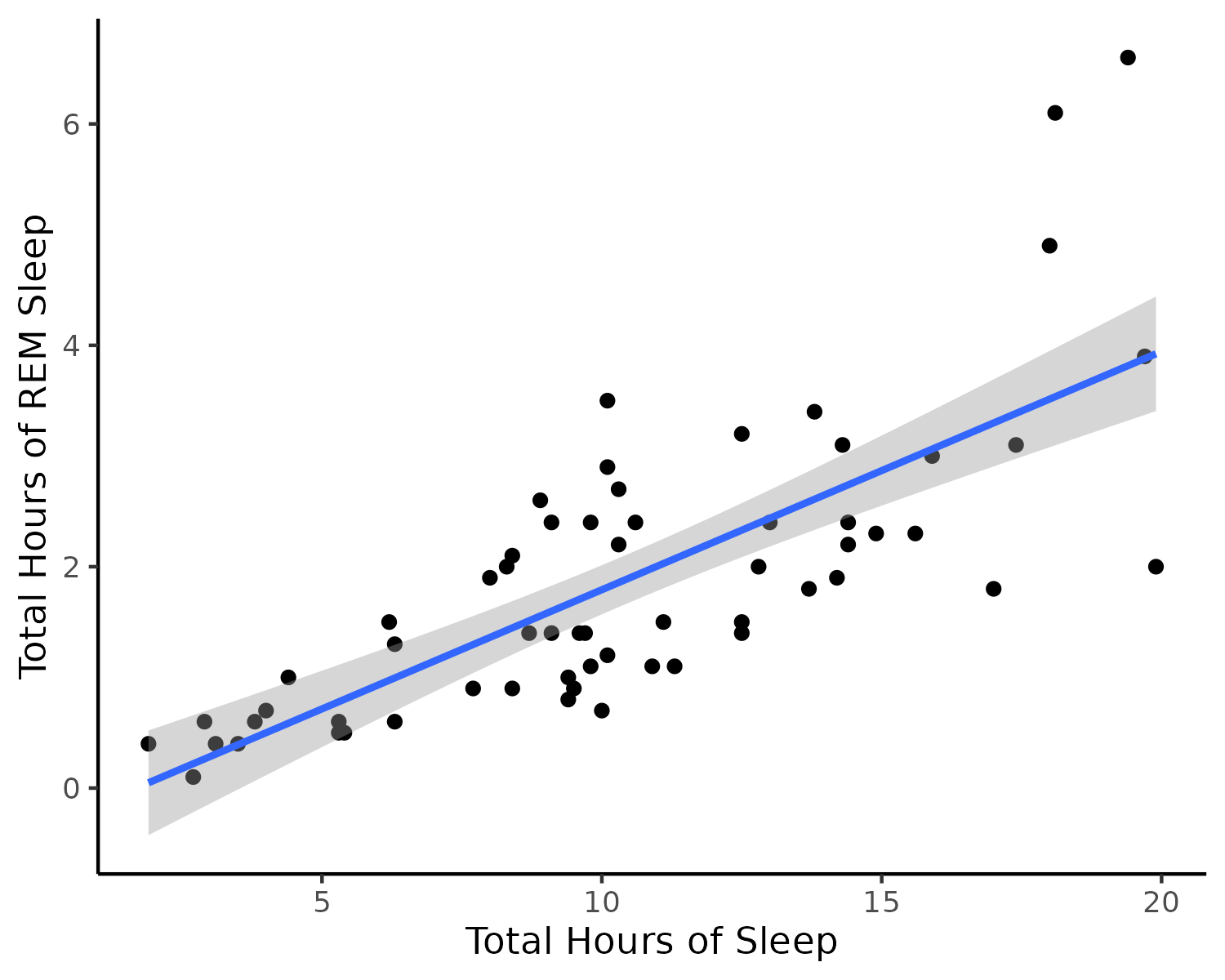 ## Workshop: Dealing with Data in R # Statistics in R ## Now that your data are ready .footnote[Steffi LaZerte <https://steffilazerte.ca> | *Compiled: 2022-01-26*] --- class: section # Basic Statistics --- # Looking at your data ```r library(skimr) skim(mtcars) ``` .small[ ``` ## ── Data Summary ──────────────────────── ## Values ## Name mtcars ## Number of rows 32 ## Number of columns 11 ## _______________________ ## Column type frequency: ## numeric 11 ## ________________________ ## Group variables None ## ## ── Variable type: numeric ──────────────────────────────────────────────────────────────────────────────────── ## skim_variable n_missing complete_rate mean sd p0 p25 p50 p75 p100 hist ## 1 mpg 0 1 20.1 6.03 10.4 15.4 19.2 22.8 33.9 ▃▇▅▁▂ ## 2 cyl 0 1 6.19 1.79 4 4 6 8 8 ▆▁▃▁▇ ## 3 disp 0 1 231. 124. 71.1 121. 196. 326 472 ▇▃▃▃▂ ## 4 hp 0 1 147. 68.6 52 96.5 123 180 335 ▇▇▆▃▁ ## 5 drat 0 1 3.60 0.535 2.76 3.08 3.70 3.92 4.93 ▇▃▇▅▁ ## 6 wt 0 1 3.22 0.978 1.51 2.58 3.32 3.61 5.42 ▃▃▇▁▂ ## 7 qsec 0 1 17.8 1.79 14.5 16.9 17.7 18.9 22.9 ▃▇▇▂▁ ## 8 vs 0 1 0.438 0.504 0 0 0 1 1 ▇▁▁▁▆ ## 9 am 0 1 0.406 0.499 0 0 0 1 1 ▇▁▁▁▆ ## 10 gear 0 1 3.69 0.738 3 3 4 4 5 ▇▁▆▁▂ ## 11 carb 0 1 2.81 1.62 1 2 2 4 8 ▇▂▅▁▁ ``` ] --- # Looking at your data ```r library(GGally) ggpairs(dplyr::select(mtcars, mpg, cyl, hp, wt, am)) ``` <img src="6 Basic Statistics_files/figure-html/unnamed-chunk-5-1.png" width="100%" style="display: block; margin: auto;" /> --- # T-Tests ### Comparing two samples ```r t.test(values ~ group, data = data) ``` - `values` are measurements from the two populations - `group` is the column that differentiates the two groups ### **OR** ```r t.test(sample1, sample2) ``` - `sample1` and `sample2` are the two samples to be compared --- # T-Tests ### Miles-per-gallon significantly different between Automatic and Manual cars? ```r ggplot(mtcars, aes(x = factor(am), y = mpg)) + geom_boxplot() ``` <img src="6 Basic Statistics_files/figure-html/unnamed-chunk-8-1.png" width="60%" style="display: block; margin: auto;" />  --- # T-Tests ### Miles-per-gallon significantly different between Automatic and Manual cars? ```r t.test(mpg ~ am, data = mtcars) ``` ``` ## ## Welch Two Sample t-test ## ## data: mpg by am ## t = -3.7671, df = 18.332, p-value = 0.001374 ## alternative hypothesis: true difference in means between group 0 and group 1 is not equal to 0 ## 95 percent confidence interval: ## -11.280194 -3.209684 ## sample estimates: ## mean in group 0 mean in group 1 ## 17.14737 24.39231 ```  --- # Other tests - Fisher's Exact Test - `fisher.test()` - Chi-Square Test - `chisq.test()` > Here it's mostly about getting your data into a matrix --- class: split-50 # Getting data into matrix for Chi-Square .columnl[ Example Data .small[ ```r my_data <- data.frame(expected = c(10, 10), observed = c(16, 4), site = c("A", "B")) my_data ``` ``` ## expected observed site ## 1 10 16 A ## 2 10 4 B ``` ] As a matrix (only expected and observed) .small[ ```r my_matrix <- dplyr::select(my_data, expected, observed) my_matrix <- as.matrix(my_matrix) my_matrix ``` ``` ## expected observed ## [1,] 10 16 ## [2,] 10 4 ``` ] ] -- .columnr[ Chi-Square Test ```r chisq.test(my_matrix) ``` ``` ## ## Pearson's Chi-squared test with Yates' continuity correction ## ## data: my_matrix ## X-squared = 2.7473, df = 1, p-value = 0.09742 ``` ] --- class: section # Non-parametric Statistics --- # Non-parametric Statistics ## Wilcoxon Rank Sum (Mann-Whitney) Test ```r air <- filter(airquality, Month %in% c(5, 8)) ``` ![:spacer 15px]() Is there a difference in air quality between May (5th month) and August (8th month)? ```r wilcox.test(Ozone ~ Month, data = air, exact = FALSE) ``` ``` ## ## Wilcoxon rank sum test with continuity correction ## ## data: Ozone by Month ## W = 127.5, p-value = 0.0001208 ## alternative hypothesis: true location shift is not equal to 0 ``` ![:spacer 15px]() Yes! --- # Non-parametric Statistics ## Kruskal-Wallis Rank Sum Test Is there a difference in air quality among months? ```r kruskal.test(Ozone ~ Month, data = airquality) ``` ``` ## ## Kruskal-Wallis rank sum test ## ## data: Ozone by Month ## Kruskal-Wallis chi-squared = 29.267, df = 4, p-value = 6.901e-06 ``` ![:spacer 15px]() Yes, there is at least one month that is different from the rest. --- class: section # Linear Models --- # Linear Models #### Running models in R ```r lm(y ~ x1 + x2, data = data) ``` - `y` is **dependent** variable - `x1` and `x2` are **independent** variables -- #### Different types of models - If both `x`'s are continuous, this is a **linear regression** - If both `x`'s are categorical, this is an **ANOVA** - If `x1` is continuous and `x2` is categorical, this is an **ANCOVA** --  --- # Linear Models: Interactions **Main effects only** ```r m <- lm(y ~ x1 + x2, data = data) ``` -- **Main effects** and **interaction** ```r m <- lm(y ~ x1 + x2 + x1:x2, data = data) ``` -- **Main effects** and **interaction** ```r m <- lm(y ~ x1 * x2, data = data) ``` -- > `x1 * x2` equivalent to `x1 + x2 + x1:x2` --- layout: true # Linear Regression #### Example with `msleep` ```r lm(sleep_cycle ~ bodywt, data = msleep) ``` ``` ## ## Call: ## lm(formula = sleep_cycle ~ bodywt, data = msleep) ## ## Coefficients: ## (Intercept) bodywt ## 0.38549 0.00107 ``` --- ---  ---  --- Hmm, not a lot of detail --- layout: false # Linear Regression #### Assign model to `m` ```r m <- lm(sleep_cycle ~ bodywt, data = msleep) ``` `m` is a model object ```r class(m) ``` ``` ## [1] "lm" ``` This contains all the information about the model --- # Linear Regression .small[ ```r summary(m) ``` ``` ## ## Call: ## lm(formula = sleep_cycle ~ bodywt, data = msleep) ## ## Residuals: ## Min 1Q Median 3Q Max ## -0.36081 -0.20228 -0.08506 0.03564 1.04817 ## ## Coefficients: ## Estimate Std. Error t value Pr(>|t|) ## (Intercept) 0.3854937 0.0623726 6.180 8.43e-07 *** ## bodywt 0.0010700 0.0004248 2.519 0.0173 * ## --- ## Signif. codes: 0 '***' 0.001 '**' 0.01 '*' 0.05 '.' 0.1 ' ' 1 ## ## Residual standard error: 0.3313 on 30 degrees of freedom ## (51 observations deleted due to missingness) ## Multiple R-squared: 0.1746, Adjusted R-squared: 0.147 ## F-statistic: 6.344 on 1 and 30 DF, p-value: 0.01734 ``` ] --  --- # Model Diagnostics ## Model Assumptions - Normality (of residuals) - Constant Variance (no heteroscedasticity) ## Other cautions - Influential variables (Cook's D) - Multiple collinearity (with more than one `x` or explanatory variables) --- # Model Diagnostics ## Diagnostics by Hand - Depending on model, different diagnostic functions (e.g., `plot()`) - But you can check any model by hand if you pull out the right data ![:spacer 5px]() First let's get our relevant variables, `residuals` and `fitted values`: ```r d <- data.frame(residuals = residuals(m), # Residuals fitted = fitted(m), # Fitted values cooks = cooks.distance(m)) # Cook's D d <- mutate(d, observation = 1:nrow(d)) # Observation number ``` -- .small[ ``` ## residuals fitted cooks observation ## 4 -0.25218072 0.3855141 1.104107e-02 1 ## 5 -0.36081280 1.0274795 1.403343e+00 2 ## 6 0.37705353 0.3896131 2.422542e-02 3 ## 7 -0.02408421 0.4074175 9.247658e-05 4 ## 9 -0.06714006 0.4004734 7.353601e-04 5 ``` ] --- class: split-50 # Normality .columnl[ #### Histogram of residuals .small[ ```r ggplot(data = d, aes(x = residuals)) + geom_histogram(bins = 20) ``` <img src="6 Basic Statistics_files/figure-html/unnamed-chunk-26-1.png" width="100%" style="display: block; margin: auto;" /> ]] .columnr[ #### QQ Normality plot of residuals .small[ ```r ggplot(data = d, aes(sample = residuals)) + stat_qq() + stat_qq_line() ``` <img src="6 Basic Statistics_files/figure-html/unnamed-chunk-27-1.png" width="100%" style="display: block; margin: auto;" /> ]] --- class: split-40 # Variance and Influence .columnl[ #### Check heteroscedasticity .small[ ```r ggplot(d, aes(x = fitted, y = residuals)) + geom_point() + geom_hline(yintercept = 0) ``` <img src="6 Basic Statistics_files/figure-html/unnamed-chunk-28-1.png" width="100%" style="display: block; margin: auto;" /> ]] .columnr[ #### Cook's D .small[ ```r ggplot(d, aes(x = observation, y = cooks)) + geom_point() + geom_hline(yintercept = 1, linetype = "dotted") + geom_hline(yintercept = 4/nrow(msleep), linetype = "dashed") ``` <img src="6 Basic Statistics_files/figure-html/unnamed-chunk-29-1.png" width="100%" style="display: block; margin: auto;" /> ]] -- .box-b[Definitely have some problems] --- class: split-40 # Diagnostics with `ggfortify` .columnl[ - Uses `autoplot` - Choose `which` plots to show - 1 = Residuals vs. fitted - 2 = QQ Norm - 4 = Cook's Distance - Others available ] .columnr[ ```r library(ggfortify) autoplot(m, which = c(1, 2, 4)) ``` <img src="6 Basic Statistics_files/figure-html/unnamed-chunk-30-1.png" width="100%" style="display: block; margin: auto;" /> ] --- # Transformations #### Let's try a log transformation - Normally you would only transform the `y` value - But mass data often works best with log10 or ln transformations (isometry) - So we'll transform both x and y here ```r msleep_log <- mutate(msleep, sleep_cycle = log10(sleep_cycle), bodywt = log10(bodywt), brainwt = log10(brainwt)) m_log <- lm(sleep_cycle ~ bodywt, data = msleep_log) ``` ![:spacer 15px]() **Note:** - By default `log()` takes the ln. Use `log10()` if you want base 10 --- # Multicollinearity (collinearity) Only relevant with more than one explanatory variable ```r m_mult <- lm(sleep_cycle ~ bodywt + brainwt, data = msleep_log) ``` -- ### Use the `car` package to get the `vif()` function ```r library(car) vif(m_mult) ``` ``` ## bodywt brainwt ## 13.30615 13.30615 ``` Hmm, that's pretty high (looking for < 10) --- # Multicollinearity (collinearity) #### Look at our two explanatory variables: ```r ggplot(data = msleep_log, aes(x = brainwt, y = bodywt)) + geom_point() + stat_smooth(method = "lm") ``` ``` ## `geom_smooth()` using formula 'y ~ x' ``` <img src="6 Basic Statistics_files/figure-html/unnamed-chunk-34-1.png" width="60%" style="display: block; margin: auto;" /> -- .box-b[Highly correlated!] --- layout: true # Interpreting linear models ```r summary(m_log) ``` .compact[.small[ ``` ## ## Call: ## lm(formula = sleep_cycle ~ bodywt, data = msleep_log) ## ## Residuals: ## Min 1Q Median 3Q Max ## -0.36819 -0.13517 -0.01879 0.05897 0.36550 ## ## Coefficients: ## Estimate Std. Error t value Pr(>|t|) ## (Intercept) -0.49439 0.03074 -16.082 2.72e-16 *** ## bodywt 0.18705 0.02197 8.515 1.68e-09 *** ## --- ## Signif. codes: 0 '***' 0.001 '**' 0.01 '*' 0.05 '.' 0.1 ' ' 1 ## ## Residual standard error: 0.1734 on 30 degrees of freedom ## (51 observations deleted due to missingness) ## Multiple R-squared: 0.7073, Adjusted R-squared: 0.6976 ## F-statistic: 72.51 on 1 and 30 DF, p-value: 1.679e-09 ``` ]] --- --- ![:hl 52%, 35%, 43%, 30px]()  --- ![:hl 78%, 59%, 190px, 75px]()  --- ![:hl 78%, 59%, 190px, 75px]()  --  --- ![:hl 78%, 59%, 190px, 75px]()  --  --- ![:hl 78%, 59%, 190px, 75px]()  --  --- ![:hl 69.5%, 59%, 100px, 75px]()  --- ![:hl 53.5%, 59%, 190px, 75px]()  --- ![:hl 53.5%, 59%, 190px, 75px]()  --- ![:hl 53.5%, 59%, 190px, 75px]()  --- ![:hl 53.5%, 59%, 190px, 75px]()  --- ![:hl 73%, 85.5%, 21%, 25px]()  --- ![:hl 48%, 85.5%, 21%, 25px]()  --- class: split-50 layout: false # ANOVAs #### Same as before, but now with categorical variables (`vore` & `conservation`) ```r m <- lm(sleep_total ~ vore + conservation, data = msleep) ``` -- #### What are these variables? .small[ .columnl[ ```r count(msleep, vore) ``` ``` ## # A tibble: 5 × 2 ## vore n ## <chr> <int> ## 1 carni 19 ## 2 herbi 32 ## 3 insecti 5 ## 4 omni 20 ## 5 <NA> 7 ``` ] .columnr[ ```r count(msleep, conservation) ``` ``` ## # A tibble: 7 × 2 ## conservation n ## <chr> <int> ## 1 cd 2 ## 2 domesticated 10 ## 3 en 4 ## 4 lc 27 ## 5 nt 4 ## 6 vu 7 ## 7 <NA> 29 ``` ]] ![:spacer 150px]() cd = conservation dependent, lc = least concern, vu = vulnerable, nt = non-threatened, en = endangered, etc. --  --- layout: true # Interpreting ANOVA *summaries* .small[ ```r summary(m) ``` ``` ## ## Call: ## lm(formula = sleep_total ~ vore + conservation, data = msleep) ## ## Residuals: ## Min 1Q Median 3Q Max ## -7.1632 -2.7702 0.2547 2.8866 6.4368 ## ## Coefficients: ## Estimate Std. Error t value Pr(>|t|) ## (Intercept) 3.851 3.041 1.266 0.21231 ## voreherbi -3.101 1.431 -2.167 0.03585 * ## voreinsecti 1.853 2.800 0.662 0.51174 ## voreomni -1.401 1.945 -0.720 0.47525 ## conservationdomesticated 6.040 3.265 1.850 0.07121 . ## conservationen 10.262 3.688 2.783 0.00797 ** ## conservationlc 9.414 3.141 2.997 0.00452 ** ## conservationnt 11.450 3.638 3.147 0.00299 ** ## conservationvu 4.407 3.353 1.314 0.19575 ## --- ``` ] --- --- ![:hl 43%, 63%, 51%, 72px]()   --  --- ![:hl 43%, 74%, 51%, 117px]()   --- layout: true # Interpreting ANOVA *tables* ```r anova(m) ``` ``` ## Analysis of Variance Table ## ## Response: sleep_total ## Df Sum Sq Mean Sq F value Pr(>F) ## vore 3 167.57 55.856 3.1960 0.032757 * ## conservation 5 342.97 68.595 3.9249 0.005095 ** ## Residuals 43 751.51 17.477 ## --- ## Signif. codes: 0 '***' 0.001 '**' 0.01 '*' 0.05 '.' 0.1 ' ' 1 ``` --- --- ![:hl 44%, 43%, 50%, 25px]()  --- ![:hl 44%, 47%, 50%, 25px]()  ---  --- layout: false class: split-50 # Interpreting ANOVA *tables* .columnl[ ## Type II ANOVA ```r library(car) Anova(m, type = "2") ``` ``` ## Anova Table (Type II tests) ## ## Response: sleep_total ## Sum Sq Df F value Pr(>F) ## vore 121.75 3 2.3220 0.088502 . ## conservation 342.97 5 3.9249 0.005095 ** ## Residuals 751.51 43 ## --- ## Signif. codes: 0 '***' 0.001 '**' 0.01 '*' 0.05 '.' 0.1 ' ' 1 ``` ] .columnr[ ## Type III ANOVA ```r library(car) Anova(m, type = "3") ``` ``` ## Anova Table (Type III tests) ## ## Response: sleep_total ## Sum Sq Df F value Pr(>F) ## (Intercept) 28.01 1 1.6029 0.212313 ## vore 121.75 3 2.3220 0.088502 . ## conservation 342.97 5 3.9249 0.005095 ** ## Residuals 751.51 43 ## --- ## Signif. codes: 0 '***' 0.001 '**' 0.01 '*' 0.05 '.' 0.1 ' ' 1 ``` ] --- class: section # ANOVAs and Post-Hoc Tests --- class: split-50 # Chicks and Diet .columnl[ ### Prep data ```r chicks <- filter(ChickWeight, Time == 21, !(Chick %in% 1:7)) head(chicks) ``` ``` ## Grouped Data: weight ~ Time | Chick ## weight Time Chick Diet ## 1 98 21 9 1 ## 2 124 21 10 1 ## 3 175 21 11 1 ## 4 205 21 12 1 ## 5 96 21 13 1 ## 6 266 21 14 1 ``` ] .columnr[ ### How many chicks per diet? ```r count(chicks, Diet) ``` ``` ## Grouped Data: weight ~ Time | Chick ## Diet n ## 1 1 9 ## 2 2 10 ## 3 3 10 ## 4 4 9 ``` ] --- class: split-50 # Chicks and Diet 4 different diets, how do chicks gain weight on each diet? ```r m <- lm(weight ~ Diet, data = chicks) ``` -- .columnl[ ```r anova(m) ``` .compact[.small[ ``` ## Analysis of Variance Table ## ## Response: weight ## Df Sum Sq Mean Sq F value Pr(>F) ## Diet 3 68673 22891.0 5.5334 0.003331 ** ## Residuals 34 140654 4136.9 ## --- ## Signif. codes: 0 '***' 0.001 '**' 0.01 '*' 0.05 '.' 0.1 ' ' 1 ``` ]] ] -- .columnr[ ```r summary(m) ``` .compact[.small[ ``` ## ## Call: ## lm(formula = weight ~ Diet, data = chicks) ## ## Residuals: ## Min 1Q Median 3Q Max ## -140.700 -39.414 -1.056 40.908 116.300 ## ## Coefficients: ## Estimate Std. Error t value Pr(>|t|) ## (Intercept) 153.33 21.44 7.152 2.87e-08 *** ## Diet2 61.37 29.55 2.077 0.045472 * ## Diet3 116.97 29.55 3.958 0.000365 *** ## Diet4 85.22 30.32 2.811 0.008143 ** ## --- ``` ]] ] --  --- # Post-Hoc Tests .medium[ ```r library(multcomp) mult_pairwise <- glht(m, linfct = mcp(Diet = "Tukey")) # All Pair-wise comparisons ``` ] - Package `multcomp` - Function `glht()` (**g**eneral **l**inear **h**ypothesis **t**esting) - Model of interest (here, **m**) - Argument `linfct` (**lin**ear **f**un**ct**ion, i.e., Which post-hoc tests?) - Function `mcp()` (**m**ultiple **c**om**p**arisons) - Specify the variable you want to compare (Here, **Diet**) - Specify the way the categories should be compared: - `"Tukey"` reflects **Tukey Contrasts** (i.e., all pairwise comparisons) - `"Dunnett"` reflects **Dunnett's comparison with a control** --- # Post-Hoc Tests ### All pair-wise comparisons .small[ ```r summary(mult_pairwise) ``` ``` ## Simultaneous Tests for General Linear Hypotheses ## ## Multiple Comparisons of Means: Tukey Contrasts ## ## ## Fit: lm(formula = weight ~ Diet, data = chicks) ## ## Linear Hypotheses: ## Estimate Std. Error t value Pr(>|t|) ## 2 - 1 == 0 61.37 29.55 2.077 0.18124 ## 3 - 1 == 0 116.97 29.55 3.958 0.00186 ** ## 4 - 1 == 0 85.22 30.32 2.811 0.03873 * ## 3 - 2 == 0 55.60 28.76 1.933 0.23359 ## 4 - 2 == 0 23.86 29.55 0.807 0.85056 ## 4 - 3 == 0 -31.74 29.55 -1.074 0.70723 ## --- ## Signif. codes: 0 '***' 0.001 '**' 0.01 '*' 0.05 '.' 0.1 ' ' 1 ## (Adjusted p values reported -- single-step method) ``` ] ![:hl 58%, 41%, 145px, 25px]()  -- ![:hl 55%, 92%, 475px, 25px]() --- # Post-Hoc Tests ### Specify the P-Value adjustment .small[ ```r summary(mult_pairwise, test = adjusted("BH")) ``` ``` ## Simultaneous Tests for General Linear Hypotheses ## ## Multiple Comparisons of Means: Tukey Contrasts ## ## ## Fit: lm(formula = weight ~ Diet, data = chicks) ## ## Linear Hypotheses: ## Estimate Std. Error t value Pr(>|t|) ## 2 - 1 == 0 61.37 29.55 2.077 0.09094 . ## 3 - 1 == 0 116.97 29.55 3.958 0.00219 ** ## 4 - 1 == 0 85.22 30.32 2.811 0.02443 * ## 3 - 2 == 0 55.60 28.76 1.933 0.09241 . ## 4 - 2 == 0 23.86 29.55 0.807 0.42515 ## 4 - 3 == 0 -31.74 29.55 -1.074 0.34837 ## --- ## Signif. codes: 0 '***' 0.001 '**' 0.01 '*' 0.05 '.' 0.1 ' ' 1 ## (Adjusted p values reported -- BH method) ``` ] ![:box 25%, 70%, 40%]("BH" = Benjamini-Hochberg,<br>also known as FDR test<br>(see <a href = "https://academic.oup.com/beheco/article/15/6/1044/206216">here for more details</a>&rpar;) ![:hl 55%, 92%, 475px, 25px]() --- class: full-width # Post-Hoc Tests .medium[ <table class="table" style="margin-left: auto; margin-right: auto;"> <thead> <tr> <th style="text-align:left;"> Argument </th> <th style="text-align:left;"> P-Value Adjustment </th> </tr> </thead> <tbody> <tr> <td style="text-align:left;font-family: monospace;"> single-step </td> <td style="text-align:left;"> Adjusted p values based on the joint normal or t distribution of the linear function </td> </tr> <tr> <td style="text-align:left;font-family: monospace;"> Shaffer </td> <td style="text-align:left;"> <a href="https://www.tandfonline.com/doi/abs/10.1080/01621459.1986.10478341">Shaffer Test</a> </td> </tr> <tr> <td style="text-align:left;font-family: monospace;"> Westfall </td> <td style="text-align:left;"> <a href="https://www.tandfonline.com/doi/abs/10.1080/01621459.1997.10473627">Westfall Test</a> </td> </tr> <tr> <td style="text-align:left;font-family: monospace;"> free </td> <td style="text-align:left;"> <a href="https://www.amazon.com/Multiple-Comparisons-Tests-Using-System/dp/1580253970">Multiple testing procedures under free combinations</a> </td> </tr> <tr> <td style="text-align:left;font-family: monospace;"> holm </td> <td style="text-align:left;"> <a href="http://www.jstor.org/stable/4615733">Holm Test</a> </td> </tr> <tr> <td style="text-align:left;font-family: monospace;"> hochberg </td> <td style="text-align:left;"> <a href="https://doi.org/10.1093/biomet/75.4.800">Hochberg Test</a> </td> </tr> <tr> <td style="text-align:left;font-family: monospace;"> hommel </td> <td style="text-align:left;"> <a href="https://doi.org/10.1093/biomet/75.2.383">Hommel Test</a> </td> </tr> <tr> <td style="text-align:left;font-family: monospace;"> bonferroni </td> <td style="text-align:left;"> Bonferroni Correction </td> </tr> <tr> <td style="text-align:left;font-family: monospace;"> BH or fdr </td> <td style="text-align:left;"> <a href="http://www.jstor.org/stable/2346101">Benjamini-Hochberg Test or False Discovery Rate Test</a> </td> </tr> <tr> <td style="text-align:left;font-family: monospace;"> BY </td> <td style="text-align:left;"> <a href="https://projecteuclid.org/euclid.aos/1013699998">Benjamini-Yekutieli Test</a> </td> </tr> <tr> <td style="text-align:left;font-family: monospace;"> none </td> <td style="text-align:left;"> No P-Value Adjustment </td> </tr> </tbody> </table> ] --- class: section # Data Transformations --- class: split-50 # Transformations .columnl[ .small[ ```r m <- lm(sleep_cycle ~ bodywt, data = msleep) d <- data.frame(residuals = residuals(m), std_residuals = rstudent(m), fitted = fitted(m), cooks = cooks.distance(m)) d <- mutate(d, observation = 1:nrow(d)) ``` ]] .columnr[ .small[ ```r ggplot(data = d, aes(sample = std_residuals)) + stat_qq() + stat_qq_line() ``` <img src="6 Basic Statistics_files/figure-html/unnamed-chunk-57-1.png" width="100%" style="display: block; margin: auto;" /> ]]  --- class: space-list # Transformations #### Order of Operations 1. See the need (e.g., non-normal residuals, heteroscedacity) 2. Figure out which transformation 3. Apply the transformation 4. Check model assumptions 5. Rinse and repeat as needed --- class: split-60 # Transformations: Common options ### Table of transformations in R .columnl[ ![:spacer 5px]() .small[ .spread[ ```r data_trans <- mutate(data, y_trans = 1/y^2) data_trans <- mutate(data, y_trans = 1/y) data_trans <- mutate(data, y_trans = 1/sqrt(y)) data_trans <- mutate(data, y_trans = log(y)) data_trans <- mutate(data, y_trans = log10(y)) data_trans <- mutate(data, y_trans = sqrt(y)) data_trans <- mutate(data, y_trans = y^2) data_trans <- mutate(data, y_trans = asin(sqrt(y/100))) data_trans <- mutate(data, y_trans = (y^lambda - 1)/lambda) ``` ]]] .columnr[ <table class="table" style="font-size: 18px; margin-left: auto; margin-right: auto;"> <thead> <tr> <th style="text-align:left;"> Transformation </th> <th style="text-align:left;"> R Code </th> </tr> </thead> <tbody> <tr> <td style="text-align:left;"> Inverse square </td> <td style="text-align:left;font-family: monospace;"> 1/y^2 </td> </tr> <tr> <td style="text-align:left;"> Reciprocal </td> <td style="text-align:left;font-family: monospace;"> 1/y </td> </tr> <tr> <td style="text-align:left;"> Inverse square root </td> <td style="text-align:left;font-family: monospace;"> 1/sqrt(y) </td> </tr> <tr> <td style="text-align:left;"> Natural log (ln) </td> <td style="text-align:left;font-family: monospace;"> log(y) </td> </tr> <tr> <td style="text-align:left;"> Log base 10 </td> <td style="text-align:left;font-family: monospace;"> log10(y) </td> </tr> <tr> <td style="text-align:left;"> Square root </td> <td style="text-align:left;font-family: monospace;"> sqrt(y) </td> </tr> <tr> <td style="text-align:left;"> Square </td> <td style="text-align:left;font-family: monospace;"> y^2 </td> </tr> <tr> <td style="text-align:left;"> Box Cox </td> <td style="text-align:left;font-family: monospace;"> (y^lambda - 1) / lambda </td> </tr> <tr> <td style="text-align:left;"> Arcsine-sqare-root </td> <td style="text-align:left;font-family: monospace;"> asin(sqrt(y/100)) </td> </tr> </tbody> </table> ]  --- class: space-list background-image: url(figures/boxcox_cropped.png) background-size: 30% background-position: bottom 0px center # Transformations: How to choose? - Based on what you know (often discipline specific standards for certain data types) - Based on what you see (does it look exponential or logarithmic?) - Based on trial and error (try different transformations and see how it goes) - Based on Box-Cox lambda `\((\lambda)\)` .center[ **Can EITHER apply `\(\lambda\)` through Box-Cox transformation OR use it to indicate best transformation**] --- class: split-50 background-image: url(figures/boxcox-1.png) background-size: 45% background-position: bottom 10px right 10px # Transformations: Find `\(\lambda\)` .columnl[ ## Plot of `\(\lambda\)` ```r library(MASS) b <- boxcox(m) ``` ## Exact `\(\lambda\)` ```r b$x[b$y == max(b$y)] ``` ``` ## [1] -0.2626263 ``` ] --- # Apply the transformation ```r msleep_trans <- mutate(msleep, sleep_cycle = (sleep_cycle^(-0.26) - 1) / -0.26) m_trans <- lm(sleep_cycle ~ bodywt, data = msleep_trans) ``` <img src="6 Basic Statistics_files/figure-html/unnamed-chunk-63-1.png" width="100%" style="display: block; margin: auto;" /> --- layout:false class: section # Generalized Linear Models --- # Generalized Linear Models ### Normal distribution - Gaussian Distribution ```r lm(y ~ x1 * x2, data = my_data) ``` ### Count data - Poisson Family ```r glm(counts ~ x1 * x2, family = "poisson", data = my_data) ``` ### Binary (0/1, Logistic Regression) - Binomial Distribution ```r glm(y ~ x1 * x2, family = "binomial", data = my_data) ``` ### Proportion with binary outcomes (10 yes, 5 no) - Binomial Distribution ```r glm(cbind(Yes, No) ~ x1 * x2, family = "binomial", data = my_data) ``` --- # Poisson - Run ### Download data ```r p <- read.csv("https://stats.idre.ucla.edu/stat/data/poisson_sim.csv") p <- mutate(p, program = factor(prog, levels = 1:3, labels = c("General", "Academic","Vocational"))) head(p) ``` ``` ## id num_awards prog math program ## 1 45 0 3 41 Vocational ## 2 108 0 1 41 General ## 3 15 0 3 44 Vocational ## 4 67 0 3 42 Vocational ## 5 153 0 3 40 Vocational ## 6 51 0 1 42 General ``` ### Run model ```r m <- glm(num_awards ~ program + math, family = "poisson", data = p) ``` --- class: split-60 # Poisson - Evaluate .columnl[ .small[ ```r summary(m) ``` ``` ## glm(formula = num_awards ~ program + math, family = "poisson", ## data = p) ## ## Deviance Residuals: ## Min 1Q Median 3Q Max ## -2.2043 -0.8436 -0.5106 0.2558 2.6796 ## ## Coefficients: ## Estimate Std. Error z value Pr(>|z|) ## (Intercept) -5.24712 0.65845 -7.969 1.60e-15 *** ## programAcademic 1.08386 0.35825 3.025 0.00248 ** ## programVocational 0.36981 0.44107 0.838 0.40179 ## math 0.07015 0.01060 6.619 3.63e-11 *** ## --- ## Signif. codes: 0 '***' 0.001 '**' 0.01 '*' 0.05 '.' 0.1 ' ' 1 ## ## (Dispersion parameter for poisson family taken to be 1) ## ## Null deviance: 287.67 on 199 degrees of freedom ## Residual deviance: 189.45 on 196 degrees of freedom ``` ]] .columnr[ Look at deviance vs. df: ```r deviance(m) ``` ``` ## [1] 189.4496 ``` ```r df.residual(m) ``` ``` ## [1] 196 ``` ```r deviance(m) / df.residual(m) ``` ``` ## [1] 0.9665797 ``` Nice! (should be close to 1) ] --- # Binary (0/1 - Logistic Regression) ### Data ```r binary <- read.csv("https://stats.idre.ucla.edu/stat/data/binary.csv") head(binary) ``` ``` ## admit gre gpa rank ## 1 0 380 3.61 3 ## 2 1 660 3.67 3 ## 3 1 800 4.00 1 ## 4 1 640 3.19 4 ## 5 0 520 2.93 4 ## 6 1 760 3.00 2 ``` ### Run model ```r m <- glm(admit ~ gpa, family = "binomial", data = binary) ``` --- class: split-60 # Binary (0/1 - Logistic Regression) .columnl[ ### Check results .small[ ```r summary(m) ``` ``` ## Call: ## glm(formula = admit ~ gpa, family = "binomial", data = binary) ## ## Deviance Residuals: ## Min 1Q Median 3Q Max ## -1.1131 -0.8874 -0.7566 1.3305 1.9824 ## ## Coefficients: ## Estimate Std. Error z value Pr(>|z|) ## (Intercept) -4.3576 1.0353 -4.209 2.57e-05 *** ## gpa 1.0511 0.2989 3.517 0.000437 *** ## --- ## Signif. codes: 0 '***' 0.001 '**' 0.01 '*' 0.05 '.' 0.1 ' ' 1 ## ## (Dispersion parameter for binomial family taken to be 1) ## ## Null deviance: 499.98 on 399 degrees of freedom ## Residual deviance: 486.97 on 398 degrees of freedom ``` ] ] .columnr[ ### Convert to Odd's Ratios ```r exp(coef(m)) ``` ``` ## (Intercept) gpa ## 0.01280926 2.86082123 ``` e.g., The odds of being admitted increase by a factor of 2.86 (x2.86 times more likely) for every unit increase in GPA. ] --- # Binary Outcomes Proportion with binary outcomes (e.g., 10 yes, 5 no) ### Get the data .small[ ```r admissions <- as.data.frame(UCBAdmissions) admissions <- spread(admissions, Admit, Freq) head(admissions) ``` ``` ## Gender Dept Admitted Rejected ## 1 Male A 512 313 ## 2 Male B 353 207 ## 3 Male C 120 205 ## 4 Male D 138 279 ## 5 Male E 53 138 ## 6 Male F 22 351 ``` ] ### Run model ```r m <- glm(cbind(Admitted, Rejected) ~ Gender, family = "binomial", data = admissions) ``` --- class: split-65 # Binary Outcomes .columnl[ ### Check results .small[ ```r summary(m) ``` ``` ## Call: ## glm(formula = cbind(Admitted, Rejected) ~ Gender, family = "binomial", ## data = admissions) ## ## Deviance Residuals: ## Min 1Q Median 3Q Max ## -16.7915 -4.7613 -0.4365 5.1025 11.2022 ## ## Coefficients: ## Estimate Std. Error z value Pr(>|z|) ## (Intercept) -0.22013 0.03879 -5.675 1.38e-08 *** ## GenderFemale -0.61035 0.06389 -9.553 < 2e-16 *** ## --- ## Signif. codes: 0 '***' 0.001 '**' 0.01 '*' 0.05 '.' 0.1 ' ' 1 ## ## (Dispersion parameter for binomial family taken to be 1) ## ## Null deviance: 877.06 on 11 degrees of freedom ## Residual deviance: 783.61 on 10 degrees of freedom ``` ] ] .columnr[ ```r deviance(m) ``` ``` ## [1] 783.607 ``` ```r df.residual(m) ``` ``` ## [1] 10 ``` ```r deviance(m) / df.residual(m) ``` ``` ## [1] 78.3607 ``` Oops, over-dispersed ] --- # Binary Outcomes ### Try again with 'quasibinomial' family .small[ ```r m <- glm(cbind(Admitted, Rejected) ~ Gender, family = "quasibinomial", data = admissions) summary(m) ``` ``` ## Call: ## glm(formula = cbind(Admitted, Rejected) ~ Gender, family = "quasibinomial", ## data = admissions) ## ## Deviance Residuals: ## Min 1Q Median 3Q Max ## -16.7915 -4.7613 -0.4365 5.1025 11.2022 ## ## Coefficients: ## Estimate Std. Error t value Pr(>|t|) ## (Intercept) -0.2201 0.3281 -0.671 0.517 ## GenderFemale -0.6104 0.5404 -1.129 0.285 ## ## (Dispersion parameter for quasibinomial family taken to be 71.52958) ## ## Null deviance: 877.06 on 11 degrees of freedom ## Residual deviance: 783.61 on 10 degrees of freedom ``` ]