NRI 7350 - Lab 5

class: title-slide, nobar

![:img right:0, bottom: 0, 65%, , ](figures/title-plot-1.png)
![:img right: 1%, top: 1%, 25%, ,](https://raw.githubusercontent.com/allisonhorst/palmerpenguins/master/man/figures/lter_penguins.png)

.footnote[Artwork by [@allison_horst](https://github.com/allisonhorst/stats-illustrations)]

## NRI 7350
# Advanced Linear Models

Transformations,   
Interactions, and  
Post-hoc tests

---
class: section

# Getting started (again)

Open RStudio  
Open your NRI project  
Open a **new** script for today:

File > New File > R Script

Make sure to load packages at the top:  
`library(tidyverse)`    
`library(palmerpenguins)`    
`library(car)`

---
class: section

# Side Note
## Messages vs. Warnings vs. Errors

---
class: space-list

# Messages and Warnings and Errors (Oh my!)

- Not all coloured text is a problem
- Messages are just helpful information

```r
ggplot(data = drop_na(penguins), aes(x = body_mass_g, y = flipper_length_mm)) +
  stat_smooth()
```

```
## `geom_smooth()` using method = 'loess' and formula 'y ~ x'
```
    
---
class: space-list

# Messages and Warnings and Errors (Oh my!)
 
- Not all coloured text is a problem
- Messages are just helpful information
- Warnings should be considered **FYIs**. They might be a problem, but not always
    - Your code will run, even with a warning
    - Warnings always start with **Warning:**

```r
ggplot(data = penguins, aes(x = sex, y = body_mass_g)) +
  geom_boxplot()
```

```
## Warning: Removed 2 rows containing non-finite values (stat_boxplot).
```

---
class: space-list

```r
ggplot(data = Penguins, aes(x = sex, y = body_mass_g)) +
  geom_boxplot()
```

```
## Error in ggplot(data = Penguins, aes(x = sex, y = body_mass_g)): object 'Penguins' not found
```

--
![:box 30%, 60%, 40%](Messages < Warnings < Errors)

---
class: section
# Data Transformations

---
class: split-50

# Transformations

## Non-normal residuals
.columnl[

```r
m <- lm(sleep_cycle ~ bodywt, data = msleep)

d <- data.frame(residuals = residuals(m),
 std_residuals = rstudent(m),
 fitted = fitted(m),
 cooks = cooks.distance(m))

d <- mutate(d, obs = 1:n())
```
]

.columnr[

```r
ggplot(data = d, aes(sample = std_residuals)) +
  stat_qq() +
  stat_qq_line()
```

<img src="5 Interactions and Post-Hoc tests - answers_files/figure-html/unnamed-chunk-5-1.png" width="90%" style="display: block; margin: auto;" />
]

![:box 75%, 75%, 45%](Use a transformation! Good for addressing non-normality of residuals, and problems with variance)

---
# Transformations

#### Order of Operations
1. See the need (i.e. non-normal residuals, heteroscedacity, etc.)
2. Figure out which transformation
3. Apply the transformation
4. Check model assumptions
5. Try again as needed

---
class: split-55
# Transformations: Common options

.columnl[
### Table of transformations in R
![:spacer 2px]()
.small[
.spread[

```r
data_trans <- mutate(data, y_trans = 1/y^2)
data_trans <- mutate(data, y_trans = 1/y)
data_trans <- mutate(data, y_trans = 1/sqrt(y))
data_trans <- mutate(data, y_trans = log(y))
data_trans <- mutate(data, y_trans = log10(y))
data_trans <- mutate(data, y_trans = sqrt(y))
data_trans <- mutate(data, y_trans = y^2)
data_trans <- mutate(data, y_trans = (y^lambda - 1)/lambda)
data_trans <- mutate(data, y_trans = asin(sqrt(y/100)))
```
]]]

.columnr[
<table class="table" style="font-size: 20px; margin-left: auto; margin-right: auto;">
 <thead>
 <tr>
 <th style="text-align:left;"> Transformation </th>
 <th style="text-align:left;"> R Code </th>
 </tr>
 </thead>
<tbody>
 <tr>
 <td style="text-align:left;"> Inverse square </td>
 <td style="text-align:left;font-family: monospace;"> 1/y^2 </td>
 </tr>
 <tr>
 <td style="text-align:left;"> Reciprocal </td>
 <td style="text-align:left;font-family: monospace;"> 1/y </td>
 </tr>
 <tr>
 <td style="text-align:left;"> Inverse square root </td>
 <td style="text-align:left;font-family: monospace;"> 1/sqrt(y) </td>
 </tr>
 <tr>
 <td style="text-align:left;"> Naural log (ln) </td>
 <td style="text-align:left;font-family: monospace;"> log(y) </td>
 </tr>
 <tr>
 <td style="text-align:left;"> Log base 10 </td>
 <td style="text-align:left;font-family: monospace;"> log10(y) </td>
 </tr>
 <tr>
 <td style="text-align:left;"> Square root </td>
 <td style="text-align:left;font-family: monospace;"> sqrt(y) </td>
 </tr>
 <tr>
 <td style="text-align:left;"> Square </td>
 <td style="text-align:left;font-family: monospace;"> y^2 </td>
 </tr>
 <tr>
 <td style="text-align:left;"> Box Cox </td>
 <td style="text-align:left;font-family: monospace;"> (y^lambda - 1) / lambda </td>
 </tr>
 <tr>
 <td style="text-align:left;"> Arcsine-sqare-root </td>
 <td style="text-align:left;font-family: monospace;"> asin(sqrt(y/100)) </td>
 </tr>
</tbody>
</table>
]

![:box 50%, 88%, 85%](<code>data_trans</code> is the NEW data frame, <code>y_trans</code> is your TRANSFORMED y-value)

---
class: split-50

# Transformations: How to choose?

- Based on what you know (often discipline specific standards for certain data types)
- Based on what you see (does it look exponential or logarithmic?)
- Based on trial and error (try different transformations and see how it goes)
- Based on Box-Cox lambda `$(\lambda)$`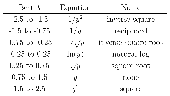

![:img right: 25px, bottom: 50px, 45%, , ](figures/boxcox_cropped.png)

![:spacer 50px]()

.columnl[
.center[
**Can EITHER**   
**Apply `$\lambda$` through Box-Cox transformation**     
**OR**    
**Use it to indicate best transformation &#8594;**  
]]

---
class: split-50

# Transformations: Box-Cox
### Finding `$\lambda$`
![:spacer 15px]()

.columnl[

- **Use a plot of `$\lambda$` **
    - `boxcox()` function from `MASS` package
    - Use `boxcox()` directly, otherwise `MASS` interferes with `select()`

```r
b <- MASS::boxcox(m) 
```
]

.columnr[
<img src="5 Interactions and Post-Hoc tests - answers_files/figure-html/unnamed-chunk-8-1.png" width="90%" style="display: block; margin: auto;" />
]

.columnl[
- **Get the exact `$\lambda$`**

```r
b$x[b$y == max(b$y)]
```

```
## [1] -0.2626263
```
]

---
# Apply the transformation

```r
msleep_trans <- mutate(msleep, sleep_cycle = (sleep_cycle^(-0.26) - 1) / -0.26)
m_trans <- lm(sleep_cycle ~ bodywt, data = msleep_trans)
```

---
class: section

# Interactions

---
# Interactions

### Interaction between Flipper Length and Species

Does the effect of Flipper Length on Body Mass depend on Species?  
(i.e. Are the slopes different?)

---
# Interactions

### Interaction between Flipper Length and Bill Length

Does the effect of Flipper Length on Body Mass depend on Bill Length?  
(i.e. Does the slope of Flipper Length change with Bill Length?)

---
# Interactions

### Main Effects only .small[\+]

### Main Effects and Interaction .small[\+ :]

### *Both* Main Effects and Interaction .small[\* (shortcut)]

![:spacer 20px]()

> Don't forget your diagnostic plots!

![:box 50%, 40%, 50%](Your turn! Create a model with your response variable by two of your continuous predictors including an interaction term. Look at the output of <code>summary(&rpar;</code>)

---
# Interpreting Interactions
### Including Correlation Tables

<code class ='r hljs remark-code'>summary(m, correlation = TRUE)</code>

.small[

```
## Coefficients:
## Estimate Std. Error t value Pr(>|t|) 
## (Intercept) 5090.5088 2925.3007 1.740 0.082740 . 
## flipper_length_mm -7.3085 15.0321 -0.486 0.627145 
## bill_length_mm -229.2424 63.4334 -3.614 0.000347 ***
## flipper_length_mm:bill_length_mm 1.1998 0.3224 3.721 0.000232 ***
## ---
## Signif. codes: 0 '***' 0.001 '**' 0.01 '*' 0.05 '.' 0.1 ' ' 1
## 
## Residual standard error: 386.8 on 338 degrees of freedom
## (2 observations deleted due to missingness)
## Multiple R-squared: 0.7694,	Adjusted R-squared: 0.7674 
## F-statistic: 375.9 on 3 and 338 DF, p-value: < 2.2e-16
## 
*## Correlation of Coefficients:
*## (Intercept) flipper_length_mm bill_length_mm
*## flipper_length_mm -1.00 
*## bill_length_mm -0.99 0.98 
*## flipper_length_mm:bill_length_mm 0.99 -0.99 -1.00
```
]

![:box 25%, 50%, 25%](But for now we'll focus on the Estimates)

---
layout: true
# Interpreting Interactions

---

```
## Coefficients:
##                                   Estimate Std. Error t value Pr(>|t|)    
## (Intercept)                      5090.5088  2925.3007   1.740 0.082740 .  
*## flipper_length_mm                  -7.3085    15.0321  -0.486 0.627145    
## bill_length_mm                   -229.2424    63.4334  -3.614 0.000347 ***
## flipper_length_mm:bill_length_mm    1.1998     0.3224   3.721 0.000232 ***
```

![:box 50%, 50%, 75%](Effect of Flipper Length on Body Mass when Bill Length is 0 mm)

![:box 50%, 65%, 75%](When Bill Length is 0 mm, Body mass decreases by 7.31 g for each 1 mm increase in Flipper Length)

![:box 50%, 65%, 75%](Not meaningful! Do we ever have a Bill Length of 0 mm? Do not interpret)

---

```
## Coefficients:
##                                   Estimate Std. Error t value Pr(>|t|)    
## (Intercept)                      5090.5088  2925.3007   1.740 0.082740 .  
## flipper_length_mm                  -7.3085    15.0321  -0.486 0.627145    
*## bill_length_mm                   -229.2424    63.4334  -3.614 0.000347 ***
## flipper_length_mm:bill_length_mm    1.1998     0.3224   3.721 0.000232 ***
```

![:box 50%, 50%, 75%](Effect of Bill Length on Body Mass when Flipper Length is 0 mm)

![:box 50%, 65%, 75%](When Flipper Length is 0 mm, Body Mass decreases by 229.24 g for each 1 mm increase in Bill Length)

![:box 50%, 65%, 75%](Not meaningful! Do we ever have a Flipper Length of 0 mm? Do not interpret)

---

![:box 50%, 50%, 50%](Change in the effect of Flipper Length on Body Mass for every 1 mm change in Bill Length)

![:box 50%, 70%, 95%](For every 1 mm increase in Bill Length, the effect of a 1 mm increase in Flipper Length on Body Mass increases by 1.2 g (i.e. the slope of the relationship between Body Mass and Flipper Length increases&rpar;)

![:box 25%, 25%, 20%](And Vice Versa!)

---

![:img center, bottom: 25px, 35%, , ](figures/wtf_allison_horst.jpeg)

.footnote[Artwork by [@allison_horst](https://github.com/allisonhorst/stats-illustrations)]

---
layout: false
# Plotting Interactions
### Create new data frame with extremes

```r
penguins_new <- expand(penguins,
 flipper_length_mm = c(min(flipper_length_mm, na.rm = TRUE),
 max(flipper_length_mm, na.rm = TRUE)),
 bill_length_mm = c(min(bill_length_mm, na.rm = TRUE),
 max(bill_length_mm, na.rm = TRUE)))
```

---
# Side Note: `tidyverse` functions

### Create new data frame with extremes

<code class ='r hljs remark-code'>penguins_new <- expand(penguins, &nbsp;&nbsp;&nbsp;&nbsp;&nbsp;&nbsp;&nbsp;&nbsp;&nbsp;&nbsp;&nbsp;&nbsp;&nbsp;&nbsp;&nbsp;&nbsp;&nbsp;&nbsp;&nbsp;&nbsp;&nbsp;&nbsp;&nbsp;flipper_length_mm = c(min(flipper_length_mm, na.rm = TRUE), &nbsp;&nbsp;&nbsp;&nbsp;&nbsp;&nbsp;&nbsp;&nbsp;&nbsp;&nbsp;&nbsp;&nbsp;&nbsp;&nbsp;&nbsp;&nbsp;&nbsp;&nbsp;&nbsp;&nbsp;&nbsp;&nbsp;&nbsp;&nbsp;&nbsp;&nbsp;&nbsp;&nbsp;&nbsp;&nbsp;&nbsp;&nbsp;&nbsp;&nbsp;&nbsp;&nbsp;&nbsp;&nbsp;&nbsp;&nbsp;&nbsp;&nbsp;&nbsp;&nbsp;&nbsp;max(flipper_length_mm, na.rm = TRUE)), &nbsp;&nbsp;&nbsp;&nbsp;&nbsp;&nbsp;&nbsp;&nbsp;&nbsp;&nbsp;&nbsp;&nbsp;&nbsp;&nbsp;&nbsp;&nbsp;&nbsp;&nbsp;&nbsp;&nbsp;&nbsp;&nbsp;&nbsp;bill_length_mm = c(min(bill_length_mm, na.rm = TRUE), &nbsp;&nbsp;&nbsp;&nbsp;&nbsp;&nbsp;&nbsp;&nbsp;&nbsp;&nbsp;&nbsp;&nbsp;&nbsp;&nbsp;&nbsp;&nbsp;&nbsp;&nbsp;&nbsp;&nbsp;&nbsp;&nbsp;&nbsp;&nbsp;&nbsp;&nbsp;&nbsp;&nbsp;&nbsp;&nbsp;&nbsp;&nbsp;&nbsp;&nbsp;&nbsp;&nbsp;&nbsp;&nbsp;&nbsp;&nbsp;&nbsp;&nbsp;max(bill_length_mm, na.rm = TRUE)))</code>

### `expand()`
- from `tidyr` package .small[(part of the `tidyverse`)]
- `tidyverse` functions always start with the **data**, followed by **other arguments**
- you can reference any column from '**data**'
- `expand()` creates a data frame with all possible combinations of new columns

---
# Plotting Interactions

### Create new data frame with extremes

### Add predicted y values

- Use `predict()` function
  - `predict()` can be used on most statistical models
- Returns predicted `body_mass_g` values for new data

```r
penguins_new <- mutate(penguins_new, body_mass_g = predict(m, newdata = penguins_new))
```

---
# Plotting Interactions

### Small data frame
- With values predicted from model
- Can plot this to illustrate interactions

```r
penguins_new
```

```
## # A tibble: 4 × 3
## flipper_length_mm bill_length_mm body_mass_g
## <int> <dbl> <dbl>
## 1 172 32.1 3099.
## 2 172 59.6 2470.
## 3 231 32.1 4941.
## 4 231 59.6 6258.
```

---
class: split-40
# Plotting Interactions

.columnl[
### Raw data (no model)
.small[

```r
ggplot(data = penguins, 
       aes(x = flipper_length_mm, 
           y = body_mass_g,
           colour = bill_length_mm)) +
  geom_point(size = 2)
```
]]

.columnr[
.small[
<img src="5 Interactions and Post-Hoc tests - answers_files/figure-html/unnamed-chunk-32-1.png" width="100%" style="display: block; margin: auto;" />
]]

---
class: split-40
# Plotting Interactions

.columnl[
### Raw data + Model interaction
.small[

```r
ggplot(data = penguins, 
       aes(x = flipper_length_mm, 
           y = body_mass_g, 
           colour = bill_length_mm)) +
  geom_point(size = 2) +
* geom_line(data = penguins_new,
*           aes(group = bill_length_mm),
*           size = 2)
```
]]

.columnr[

<img src="5 Interactions and Post-Hoc tests - answers_files/figure-html/unnamed-chunk-33-1.png" width="100%" style="display: block; margin: auto;" />
]

---
class: split-50
# Plotting Interactions
.columnl[
### From a Flipper Length perspective
.small[

```r
ggplot(data = penguins, aes(x = flipper_length_mm, 
                            y = body_mass_g, 
                            colour = bill_length_mm, 
                            group = bill_length_mm)) +
  geom_point() +
  geom_line(data = penguins_new, size = 2)
```

<img src="5 Interactions and Post-Hoc tests - answers_files/figure-html/unnamed-chunk-34-1.png" width="90%" style="display: block; margin: auto;" />
]
]

.columnr[
### From a Bill Length perspective
.compact[.small[

```r
ggplot(data = penguins, aes(x = bill_length_mm, 
                            y = body_mass_g, 
                            colour = flipper_length_mm, 
                            group = flipper_length_mm))+
  geom_point() +
  geom_line(data = penguins_new, size = 2)
```

<img src="5 Interactions and Post-Hoc tests - answers_files/figure-html/unnamed-chunk-35-1.png" width="90%" style="display: block; margin: auto;" />
]]]

---
# Visualizing Interactions

Not what you would present in a paper, but good to think about
<img src="5 Interactions and Post-Hoc tests - answers_files/figure-html/unnamed-chunk-36-1.png" width="100%" style="display: block; margin: auto;" />

---
class: section
# ANOVAs and Post-Hoc Tests

---
# Post-Hoc Tests

### From last week...

```r
Anova(m, type = 3)
```

```
## Anova Table (Type III tests)
## 
## Response: body_mass_g
## Sum Sq Df F value Pr(>F) 
## (Intercept) 1154266972 1 11514.96 < 2.2e-16 ***
## species 143401584 2 715.29 < 2.2e-16 ***
## sex 37090262 1 370.01 < 2.2e-16 ***
## Residuals 32979185 329 
## ---
## Signif. codes: 0 '***' 0.001 '**' 0.01 '*' 0.05 '.' 0.1 ' ' 1
```

Differences within groups, but how are they different?

---
class: split-50
# Post-Hoc Tests

.columnl[
- Males significantly bigger than females
- Only two groups, so we can use the figure
]
.columnr[
- Are Adelie and Chinstrap the same size?
- Looks like it, but no statistical support
]

![:box 45%, 40%, 40%](Use post-hoc tests to test each combination against the others)

---
# Estimated Marginal Means

### `emmeans()` function from `emmeans` package
- Calculates **estimated marginal means** (least-squares means) 
- Mean response of each factor, adjusting for other factors
- Can think of this as a predicted mean response if sample sizes were equal  
  (and controlling for other parameters)

```r
library(emmeans)
emm_sp <- emmeans(m, specs = "species")
emm_sp
```

```
##  species   emmean   SE  df lower.CL upper.CL
##  Adelie      3706 26.2 329     3655     3758
##  Chinstrap   3733 38.4 329     3658     3809
##  Gentoo      5084 29.0 329     5027     5141
## 
*## Results are averaged over the levels of: sex 
## Confidence level used: 0.95
```

---
class: split-35, space-list
layout: true
# Post-Hoc Tests .small[(All pair-wise)]

### `pairs()` function from `emmeans` packages

.columnl[
- Compare each combination

```r
pairs(emm_sp)
```
]

---
.columnr[
![:spacer 10px]()
.medium[

```
## contrast estimate SE df t.ratio p.value
## Adelie - Chinstrap -26.9 46.5 329 -0.579 0.8313 
## Adelie - Gentoo -1377.9 39.1 329 -35.236 <.0001 
## Chinstrap - Gentoo -1350.9 48.1 329 -28.067 <.0001 
## 
## Results are averaged over the levels of: sex 
## P value adjustment: tukey method for comparing a family of 3 estimates
```
]]

---
.columnr[
![:spacer 10px]()
.medium[

```
## contrast estimate SE df t.ratio p.value
*## Adelie - Chinstrap -26.9 46.5 329 -0.579 0.8313 
## Adelie - Gentoo -1377.9 39.1 329 -35.236 <.0001 
## Chinstrap - Gentoo -1350.9 48.1 329 -28.067 <.0001 
## 
## Results are averaged over the levels of: sex 
## P value adjustment: tukey method for comparing a family of 3 estimates
```
]]

.columnl[
**Differences in Body Mass**
.medium[
- Adelie penguins are **not** different from Chinstrap penguins   
   (P value = 0.831)
]]

---
.columnr[
![:spacer 10px]()
.medium[

```
## contrast estimate SE df t.ratio p.value
## Adelie - Chinstrap -26.9 46.5 329 -0.579 0.8313 
*## Adelie - Gentoo -1377.9 39.1 329 -35.236 <.0001 
## Chinstrap - Gentoo -1350.9 48.1 329 -28.067 <.0001 
## 
## Results are averaged over the levels of: sex 
## P value adjustment: tukey method for comparing a family of 3 estimates
```
]]

.columnl[
**Differences in Body Mass**
.medium[
- Adelie penguins are **not** different from Chinstrap penguins 
 (P value = 0.831)
- Adelie penguins **are** on average 1377.9 g lighter than Gentoo penguins (P value = < 0.0001)
]]

---
.columnr[
![:spacer 10px]()
.medium[

```
## contrast estimate SE df t.ratio p.value
## Adelie - Chinstrap -26.9 46.5 329 -0.579 0.8313 
## Adelie - Gentoo -1377.9 39.1 329 -35.236 <.0001 
*## Chinstrap - Gentoo -1350.9 48.1 329 -28.067 <.0001 
## 
## Results are averaged over the levels of: sex 
## P value adjustment: tukey method for comparing a family of 3 estimates
```
]]

.columnl[
**Differences in Body Mass**
.medium[
- Adelie penguins are **not** different from Chinstrap penguins 
 (P value = 0.831)
- Adelie penguins **are** on average 1377.9 g lighter than Gentoo penguins (P value = < 0.0001)
- Chinstrap penguins **are** on average 1350.9 g lighter than Gentoo penguins (P value < 0.0001)
]]

![:box 35%, 65%, 40%](Therefore, on average Gentoo penguins are the largest Adelie and Chinstrap penguins are the same size)

---
layout: false
# Post-Hoc Tests .small[(Dunnett's)]

### With `contrast()` function from `emmeans` package
- Dunnett's comparison is a type of contrast
- Each level compared to control
- Use `method = "trt.vs.ctrl"` OR `method = "dunnett"`

```r
contrast(emm_sp, method = "dunnett")
```

```
## contrast estimate SE df t.ratio p.value
## Chinstrap - Adelie 26.9 46.5 329 0.579 0.7753 
## Gentoo - Adelie 1377.9 39.1 329 35.236 <.0001 
## 
## Results are averaged over the levels of: sex 
## P value adjustment: dunnettx method for 2 tests
```

> Look familiar?

---
class: split-50
# Post-Hoc Tests .small[(Dunnett's)]

### Dunnett's treatment vs. control contrasts with `summary()` table

.small[

```r
summary(m)
```

```
## Coefficients:
## Estimate Std. Error t value Pr(>|t|) 
## (Intercept) 3372.39 31.43 107.308 <2e-16 ***
*## speciesChinstrap 26.92 46.48 0.579 0.563 
*## speciesGentoo 1377.86 39.10 35.236 <2e-16 ***
*## sexmale 667.56 34.70 19.236 <2e-16 ***
```
]

### Dunnett's treatment vs. control contrasts with `emmeans`
![:spacer 5px]()
.columnl[
.small[

```r
contrast(emm_sp, method = "dunnett", adjust = "none")
```

```
## contrast estimate SE df t.ratio p.value
*## Chinstrap - Adelie 26.9 46.5 329 0.579 0.5628 
*## Gentoo - Adelie 1377.9 39.1 329 35.236 <.0001 
## 
## Results are averaged over the levels of: sex
```
]]

.columnr[
.small[

```r
contrast(emmeans(m, specs = "sex"), method = "dunnett", 
         adjust = "none")
```

```
## contrast estimate SE df t.ratio p.value
*## male - female 668 34.7 329 19.236 <.0001 
## 
## Results are averaged over the levels of: species
```
]]

---
class: split-50
# Post-Hoc Tests and P-Value adjustments

.footnote[\* Don't use "Bonferroni, [see this article](https://academic.oup.com/beheco/article/15/6/1044/206216)]

.columnl[
### No adjustment, too liberal?

```r
pairs(emm_sp, adjust = "none")
```

.small[

```
## contrast estimate SE df t.ratio p.value
## Adelie - Chinstrap -26.9 46.5 329 -0.579 0.5628 
## Adelie - Gentoo -1377.9 39.1 329 -35.236 <.0001 
## Chinstrap - Gentoo -1350.9 48.1 329 -28.067 <.0001 
## 
## Results are averaged over the levels of: sex
```

]
]

.columnr[
### Extremely conservative\*

```r
pairs(emm_sp, adjust = "bonferroni")
```

.small[

```
## contrast estimate SE df t.ratio p.value
## Adelie - Chinstrap -26.9 46.5 329 -0.579 1.0000 
## Adelie - Gentoo -1377.9 39.1 329 -35.236 <.0001 
## Chinstrap - Gentoo -1350.9 48.1 329 -28.067 <.0001 
## 
## Results are averaged over the levels of: sex 
## P value adjustment: bonferroni method for 3 tests
```

]
]

![:box 50%, 75%, 50%](In these examples, little difference, but can make a HUGE difference in other analyses)

---
# Post-Hoc Tests and P-Value adjustments

### Middle of the road: Benjamini Hochberg (FDR, False Discovery Rate)\*

```r
pairs(emm_sp, adjust = "fdr")
```

.footnote[\* [See this article](https://academic.oup.com/beheco/article/15/6/1044/206216)]

--
> **No one best method**   
> What is your question? Are you more concerned about Type 1 or Type 2 error?

---
class: medium-table
# Post-Hoc Tests

### Test options

<table class="table" style="margin-left: auto; margin-right: auto;">
 <thead>
 <tr>
 <th style="text-align:left;"> Argument </th>
 <th style="text-align:left;"> P-Value Adjustment </th>
 </tr>
 </thead>
<tbody>
 <tr>
 <td style="text-align:left;font-family: monospace;"> none </td>
 <td style="text-align:left;"> No P-Value Adjustment (essentially Fisher's LSD) </td>
 </tr>
 <tr>
 <td style="text-align:left;font-family: monospace;"> tukey </td>
 <td style="text-align:left;"> Tukey's HSD (Honestly significant difference), uses the Studentized range distribution with the number of means in the family. </td>
 </tr>
 <tr>
 <td style="text-align:left;font-family: monospace;"> fdr </td>
 <td style="text-align:left;"> <a href="http://www.jstor.org/stable/2346101">Benjamini-Hochberg Test or False Discovery Rate Test</a> </td>
 </tr>
 <tr>
 <td style="text-align:left;font-family: monospace;"> bonferroni </td>
 <td style="text-align:left;"> Bonferroni Correction </td>
 </tr>
 <tr>
 <td style="text-align:left;font-family: monospace;"> scheffe </td>
 <td style="text-align:left;"> Computes p values from F distribution </td>
 </tr>
 <tr>
 <td style="text-align:left;font-family: monospace;"> mvt </td>
 <td style="text-align:left;"> Adjusted p values based on the joint normal or t distribution of the linear function </td>
 </tr>
 <tr>
 <td style="text-align:left;font-family: monospace;"> holm </td>
 <td style="text-align:left;"> <a href="http://www.jstor.org/stable/4615733">Holm Test</a> </td>
 </tr>
 <tr>
 <td style="text-align:left;font-family: monospace;"> hochberg </td>
 <td style="text-align:left;"> <a href="https://doi.org/10.1093/biomet/75.4.800">Hochberg Test</a> </td>
 </tr>
 <tr>
 <td style="text-align:left;font-family: monospace;"> hommel </td>
 <td style="text-align:left;"> <a href="https://doi.org/10.1093/biomet/75.2.383">Hommel Test</a> </td>
 </tr>
</tbody>
</table>

---
# Post-Hoc Tests with Interactions

### Model: 2-way ANOVA

```r
m <- lm(body_mass_g ~ species * sex, data = penguins)
```

### Estimated Marginal Means

```r
library(emmeans)
m_emms <- emmeans(m, specs = c("species", "sex"))
m_emms
```

```
##  species   sex    emmean   SE  df lower.CL upper.CL
##  Adelie    female   3369 36.2 327     3298     3440
##  Chinstrap female   3527 53.1 327     3423     3632
##  Gentoo    female   4680 40.6 327     4600     4760
##  Adelie    male     4043 36.2 327     3972     4115
##  Chinstrap male     3939 53.1 327     3835     4043
##  Gentoo    male     5485 39.6 327     5407     5563
## 
## Confidence level used: 0.95
```

---
class: split-35, space-list
layout: true
# Post-Hoc Tests with Interactions .small[(All pair-wise)]

### `pairs()` function from `emmeans` packages

.columnl[
- Compare each combination

```r
pairs(m_emms, adjust = "fdr")
```
]

---
.columnr[
![:spacer 10px]()
.small[

```
## contrast estimate SE df t.ratio p.value
## Adelie female - Chinstrap female -158 64.2 327 -2.465 0.0152 
## Adelie female - Gentoo female -1311 54.4 327 -24.088 <.0001 
## Adelie female - Adelie male -675 51.2 327 -13.174 <.0001 
## Adelie female - Chinstrap male -570 64.2 327 -8.875 <.0001 
## Adelie female - Gentoo male -2116 53.7 327 -39.425 <.0001 
## Chinstrap female - Gentoo female -1153 66.8 327 -17.246 <.0001 
## Chinstrap female - Adelie male -516 64.2 327 -8.037 <.0001 
## Chinstrap female - Chinstrap male -412 75.0 327 -5.487 <.0001 
## Chinstrap female - Gentoo male -1958 66.2 327 -29.564 <.0001 
## Gentoo female - Adelie male 636 54.4 327 11.691 <.0001 
## Gentoo female - Chinstrap male 741 66.8 327 11.085 <.0001 
## Gentoo female - Gentoo male -805 56.7 327 -14.188 <.0001 
## Adelie male - Chinstrap male 105 64.2 327 1.627 0.1047 
## Adelie male - Gentoo male -1441 53.7 327 -26.855 <.0001 
## Chinstrap male - Gentoo male -1546 66.2 327 -23.345 <.0001 
## 
## P value adjustment: fdr method for 15 tests
```
]]

---
.columnr[
![:spacer 10px]()
.small[

```
## contrast estimate SE df t.ratio p.value
*## Adelie female - Chinstrap female -158 64.2 327 -2.465 0.0152 
## Adelie female - Gentoo female -1311 54.4 327 -24.088 <.0001 
## Adelie female - Adelie male -675 51.2 327 -13.174 <.0001 
## Adelie female - Chinstrap male -570 64.2 327 -8.875 <.0001 
## Adelie female - Gentoo male -2116 53.7 327 -39.425 <.0001 
## Chinstrap female - Gentoo female -1153 66.8 327 -17.246 <.0001 
## Chinstrap female - Adelie male -516 64.2 327 -8.037 <.0001 
## Chinstrap female - Chinstrap male -412 75.0 327 -5.487 <.0001 
## Chinstrap female - Gentoo male -1958 66.2 327 -29.564 <.0001 
## Gentoo female - Adelie male 636 54.4 327 11.691 <.0001 
## Gentoo female - Chinstrap male 741 66.8 327 11.085 <.0001 
## Gentoo female - Gentoo male -805 56.7 327 -14.188 <.0001 
## Adelie male - Chinstrap male 105 64.2 327 1.627 0.1047 
## Adelie male - Gentoo male -1441 53.7 327 -26.855 <.0001 
## Chinstrap male - Gentoo male -1546 66.2 327 -23.345 <.0001 
## 
## P value adjustment: fdr method for 15 tests
```
]]

.columnl[
**Differences in Body Mass**
.medium[
- Female Adelie penguins **are** on average 158 g smaller than female Chinstrap penguins (P value = 0.015)
]]

---
.columnr[
![:spacer 10px]()
.small[

```
## contrast estimate SE df t.ratio p.value
## Adelie female - Chinstrap female -158 64.2 327 -2.465 0.0152 
## Adelie female - Gentoo female -1311 54.4 327 -24.088 <.0001 
## Adelie female - Adelie male -675 51.2 327 -13.174 <.0001 
## Adelie female - Chinstrap male -570 64.2 327 -8.875 <.0001 
## Adelie female - Gentoo male -2116 53.7 327 -39.425 <.0001 
## Chinstrap female - Gentoo female -1153 66.8 327 -17.246 <.0001 
## Chinstrap female - Adelie male -516 64.2 327 -8.037 <.0001 
## Chinstrap female - Chinstrap male -412 75.0 327 -5.487 <.0001 
## Chinstrap female - Gentoo male -1958 66.2 327 -29.564 <.0001 
## Gentoo female - Adelie male 636 54.4 327 11.691 <.0001 
## Gentoo female - Chinstrap male 741 66.8 327 11.085 <.0001 
## Gentoo female - Gentoo male -805 56.7 327 -14.188 <.0001 
*## Adelie male - Chinstrap male 105 64.2 327 1.627 0.1047 
## Adelie male - Gentoo male -1441 53.7 327 -26.855 <.0001 
## Chinstrap male - Gentoo male -1546 66.2 327 -23.345 <.0001 
## 
## P value adjustment: fdr method for 15 tests
```
]]

.columnl[
**Differences in Body Mass**
.medium[
- Female Adelie penguins **are** on average 158 g smaller than female Chinstrap penguins (P value = 0.015)
- Male Adelie penguins are **not** different from male Chinstrap penguins (P value = 0.105)
]]

---
.columnr[
![:spacer 10px]()
.small[

```
## contrast estimate SE df t.ratio p.value
## Adelie female - Chinstrap female -158 64.2 327 -2.465 0.0152 
## Adelie female - Gentoo female -1311 54.4 327 -24.088 <.0001 
*## Adelie female - Adelie male -675 51.2 327 -13.174 <.0001 
## Adelie female - Chinstrap male -570 64.2 327 -8.875 <.0001 
## Adelie female - Gentoo male -2116 53.7 327 -39.425 <.0001 
## Chinstrap female - Gentoo female -1153 66.8 327 -17.246 <.0001 
## Chinstrap female - Adelie male -516 64.2 327 -8.037 <.0001 
## Chinstrap female - Chinstrap male -412 75.0 327 -5.487 <.0001 
## Chinstrap female - Gentoo male -1958 66.2 327 -29.564 <.0001 
## Gentoo female - Adelie male 636 54.4 327 11.691 <.0001 
## Gentoo female - Chinstrap male 741 66.8 327 11.085 <.0001 
## Gentoo female - Gentoo male -805 56.7 327 -14.188 <.0001 
## Adelie male - Chinstrap male 105 64.2 327 1.627 0.1047 
## Adelie male - Gentoo male -1441 53.7 327 -26.855 <.0001 
## Chinstrap male - Gentoo male -1546 66.2 327 -23.345 <.0001 
## 
## P value adjustment: fdr method for 15 tests
```
]]

---
layout: false
class: split-70, space-list
# Post-Hoc Tests with Interactions

.columnl[
### Model: ANCOVA

```r
m <- lm(body_mass_g ~ flipper_length_mm * species, data = penguins)
```

### Estimated Marginal Means

- Here use `emtrends()` function from `emmeans` package

```r
m_emms <- emtrends(m, specs = "species", var = "flipper_length_mm")
m_emms
```

.small[

```
##  species   flipper_length_mm.trend   SE  df lower.CL upper.CL
##  Adelie                       32.8 4.63 336     23.7     41.9
##  Chinstrap                    34.6 6.35 336     22.1     47.1
##  Gentoo                       54.6 5.17 336     44.4     64.8
## 
## Confidence level used: 0.95
```

]

These are the effects of Flipper Length on Body Mass in each Species.
]

.columnr[
.medium[
**On average...**

- Adelie: Body Mass increases by 32.8 g for each 1 mm increase in Flipper Length.
- Chinstrap: Body Mass increases by 34.6 g for each 1 mm increase in Flipper Length.
- Gentoo: Body Mass increases by 54.6 g for each 1 mm increase in Flipper Length.
]]

![:box 17%, 75%, 20%](But are these different from one another?)

---
class: split-35, space-list
layout: true
# Post-Hoc Tests with Interactions .small[(All pair-wise)]

### `pairs()` function from `emmeans` packages

.columnl[
- Compare among species

```r
pairs(m_emms, adjust = "fdr")
```
]

---
.columnr[
![:spacer 10px]()
.small[

```
##  contrast           estimate   SE  df t.ratio p.value
##  Adelie - Chinstrap    -1.74 7.86 336 -0.222  0.8247 
##  Adelie - Gentoo      -21.79 6.94 336 -3.139  0.0055 
##  Chinstrap - Gentoo   -20.05 8.19 336 -2.448  0.0223 
## 
## P value adjustment: fdr method for 3 tests
```
]]

---
.columnr[
![:spacer 10px]()
.small[

```
##  contrast           estimate   SE  df t.ratio p.value
*##  Adelie - Chinstrap    -1.74 7.86 336 -0.222  0.8247 
##  Adelie - Gentoo      -21.79 6.94 336 -3.139  0.0055 
##  Chinstrap - Gentoo   -20.05 8.19 336 -2.448  0.0223 
## 
## P value adjustment: fdr method for 3 tests
```
]]

![:spacer 100px]()

**Differences in the effect of Flipper Length on Body Mass**
.medium[
- The effect of Flipper Length on Body Mass is **not** different between Adelie and Chinstrap penguins (P value = 0.825)
]

---
.columnr[
![:spacer 10px]()
.small[

```
##  contrast           estimate   SE  df t.ratio p.value
##  Adelie - Chinstrap    -1.74 7.86 336 -0.222  0.8247 
*##  Adelie - Gentoo      -21.79 6.94 336 -3.139  0.0055 
##  Chinstrap - Gentoo   -20.05 8.19 336 -2.448  0.0223 
## 
## P value adjustment: fdr method for 3 tests
```
]]

![:spacer 100px]()

---
.columnr[
![:spacer 10px]()
.small[

```
##  contrast           estimate   SE  df t.ratio p.value
##  Adelie - Chinstrap    -1.74 7.86 336 -0.222  0.8247 
##  Adelie - Gentoo      -21.79 6.94 336 -3.139  0.0055 
*##  Chinstrap - Gentoo   -20.05 8.19 336 -2.448  0.0223 
## 
## P value adjustment: fdr method for 3 tests
```
]]

![:spacer 100px]()

**Differences in the effect of Flipper Length on Body Mass**
.medium[
- The effect of Flipper Length on Body Mass is **not** different between Adelie and Chinstrap penguins (P value = 0.825)
- The effect of Flipper Length on Body Mass **is significantly less** in Adelie than in Gentoo penguins (Body Mass increases 21.8 g less per 1mm increase in Flipper Length; P value = 0.006)
- The effect of Flipper Length on Body Mass **is significantly less** in Chinstrap than in Gentoo penguins (Body Mass increases 20 g less per 1mm increase in Flipper Length; P value = 0.022)
]

![:box 50%, 50%, 50%](Best way is to use a figure at the same time!)

---
layout: false
class: split-40, space-list
# Visualizing Interactions

```r
emmip(m, species ~ flipper_length_mm, cov.reduce = range)
```

.columnl[
.medium[
- Here, **Linear prediction** = **y** = **Body Mass**
- Adelie and Chinstrap penguins have similar effects (i.e. slopes are **not** significantly different)
- Gentoo has a larger effect (i.e. slope **is** significantly larger) than either Adelie or Chinstrap penguins
]]
.columnr[
<img src="5 Interactions and Post-Hoc tests - answers_files/figure-html/unnamed-chunk-66-1.png" width="100%" style="display: block; margin: auto;" />
]

---
# Homework (Practice)*

Consider bill depth your response variable and species and year your predictor variables

1\. Convert year to a categorical variable and remove Gentoo penguins

```r
penguins_sub <- mutate(penguins, year = factor(year))
penguins_sub <- filter(penguins_sub, species != "Gentoo")
```

2\. Create a figure comparing bill depth to species and year. Think about how to best tease apart the relationships.

3\. Model the relationship between bill depth and the interaction between species and year.

4\. Check diagnostics

5\. How does the relationship of species and bill depth change among years?

.footnote[\* Not to be handed in, answers posted in these slides next week]

---
exclude: FALSE
# Homework (Practice) Answers

2\. Create a figure comparing body mass to bill depth and year

```r
ggplot(penguins_sub, aes(x = bill_depth_mm, y = body_mass_g, colour = year)) +
  geom_point() +
  stat_smooth(method = "lm", se = FALSE)
```

---
exclude: FALSE
class: split-50
# Homework (Practice) Answers

3\. Model the relationship between body mass and the interaction between bill depth and year.

```r
m <- lm(body_mass_g ~ bill_depth_mm * year, data = penguins_sub)
```

---
exclude: FALSE
# Homework (Practice) Answers

4\. Check your model diagnostics

```r
d <- data.frame(residuals = residuals(m), 
 std_residuals = rstudent(m), 
 fitted = fitted(m), 
 cooks = cooks.distance(m))

d <- mutate(d, obs = 1:n())
d
```

```
##       residuals std_residuals   fitted        cooks obs
## 1     48.767953   0.139759238 3701.232 4.422779e-05   1
## 2    334.691697   0.969259197 3465.308 4.778239e-03   2
## 3   -324.196185  -0.933081958 3574.196 2.640006e-03   3
## 5   -360.119929  -1.036704430 3810.120 3.161623e-03   4
## 6   -396.043674  -1.160886854 4046.044 1.204535e-02   5
## 7     87.099776   0.250606023 3537.900 2.251416e-04   6
## 8    810.436130   2.363323737 3864.564 2.057554e-02   7
## 9   -117.344165  -0.336917273 3592.344 3.208236e-04   8
## 10   276.548248   0.803388875 3973.452 4.139380e-03   9
## 11  -110.864362  -0.321859240 3410.864 6.887368e-04  10
## 12   252.839677   0.732531214 3447.160 2.988740e-03  11
## 13  -301.604264  -0.870950455 3501.604 3.229564e-03  12
## 14  -354.931556  -1.054939693 4154.932 1.568554e-02  13
## 15   263.216425   0.779297638 4136.784 7.985436e-03  14
## 16   162.099776   0.466568506 3537.900 7.798057e-04  15
## 17  -305.675988  -0.878044715 3755.676 1.884339e-03  16
## 18   435.808346   1.281026324 4064.192 1.586371e-02  17
## 19  -321.788106  -0.924333210 3646.788 2.032933e-03  18
## 20    -9.375497  -0.028041477 4209.375 1.370199e-05  19
## 21  -228.640126  -0.656327379 3628.640 1.074801e-03  20
## 22  -101.232047  -0.290155114 3701.232 1.905734e-04  21
## 23     8.028051   0.023038881 3791.972 1.461514e-06  22
## 24   357.655835   1.029184148 3592.344 2.980395e-03  23
## 25   370.987658   1.078009849 3429.012 7.047852e-03  24
## 26    62.471992   0.179085488 3737.528 7.552857e-05  25
## 27  -133.084067  -0.381513303 3683.084 3.303557e-04  26
## 28  -356.048205  -1.025953499 3556.048 3.453529e-03  27
## 29  -533.084067  -1.536151293 3683.084 5.300552e-03  28
## 30   212.471992   0.609570790 3737.528 8.736630e-04  29
## 31   -88.272441  -0.258174262 3338.272 6.182483e-04  30
## 32   307.655835   0.884730440 3592.344 2.205330e-03  31
## 33  -237.900224  -0.685149423 3537.900 1.679621e-03  32
## 34   162.471992   0.465953919 3737.528 5.108549e-04  33
## 35   -67.716382  -0.196897903 3392.716 2.808596e-04  34
## 36    13.216425   0.039073721 4136.784 2.013264e-05  35
## 37    12.844208   0.037145335 3937.156 7.444577e-06  36
## 38  -114.936087  -0.329499854 3664.936 2.509617e-04  37
## 39  -510.119929  -1.472281952 3810.120 6.343958e-03  38
## 40   876.176031   2.551501243 3773.824 1.633167e-02  39
## 41  -424.196185  -1.222684981 3574.196 4.519836e-03  40
## 42   253.211894   0.726791217 3646.788 1.258784e-03  41
## 43  -564.936087  -1.629254760 3664.936 6.063081e-03  42
## 44   517.288149   1.498365968 3882.712 9.171684e-03  43
## 45  -374.568401  -1.094081198 3374.568 9.380741e-03  44
## 46   880.619972   2.562562573 3719.380 1.460218e-02  45
## 47  -330.675988  -0.950150633 3755.676 2.205168e-03  46
## 48  -762.528008  -2.210789611 3737.528 1.125258e-02  47
## 49  -106.048205  -0.304889117 3556.048 3.063741e-04  48
## 50    -4.931556  -0.014619423 4154.932 3.028155e-06  49
## 51  -106.584816  -0.306245393 3606.585 2.895658e-04  50
## 52   370.510222   1.067755506 3929.490 3.706662e-03  51
## 53  -210.402309  -0.604311787 3660.402 9.998535e-04  52
## 54   -40.942259  -0.118418323 4090.942 7.607157e-05  53
## 55  -814.219803  -2.365854800 3714.220 1.389170e-02  54
## 56  -148.763537  -0.427056698 3848.764 4.948293e-04  55
## 57    -2.767322  -0.007961092 3552.767 2.274088e-07  56
## 58  -102.581031  -0.294699802 3902.581 2.644484e-04  57
## 59  -460.588600  -1.347050783 3310.589 1.406919e-02  58
## 60  -233.307271  -0.672372159 3983.307 1.727471e-03  59
## 61  -241.314841  -0.699974231 3391.315 2.949859e-03  60
## 62  -121.482208  -0.365064049 4521.482 2.538871e-03  61
## 63   181.776412   0.526234083 3418.224 1.527973e-03  62
## 64   308.871450   0.887396567 3741.129 1.966182e-03  63
## 65  -595.132335  -1.731540709 3445.132 1.495024e-02  64
## 66   262.688944   0.754592546 3687.311 1.491376e-03  65
## 67   147.046387   0.432083005 3202.954 2.020754e-03  66
## 68   116.692729   0.336030195 3983.307 4.321574e-04  67
## 69  -260.588600  -0.759917060 3310.589 4.503535e-03  68
## 70   385.966488   1.118101105 4064.034 6.171361e-03  69
## 71  -356.398524  -1.027669655 3956.399 3.709107e-03  70
## 72   105.053957   0.301354913 3794.946 2.301925e-04  71
## 73    77.958919   0.224982615 3472.041 2.342879e-04  72
## 74   220.510222   0.634377122 3929.490 1.312925e-03  73
## 75   147.232678   0.423741436 3552.767 6.437190e-04  74
## 76   428.145210   1.232551969 3821.855 3.932187e-03  75
## 77   335.593906   0.976054439 3364.406 6.246589e-03  76
## 78  -164.033512  -0.474042597 4064.034 1.114672e-03  77
## 79   373.955134   1.104200180 3176.045 1.419206e-02  78
## 80    16.692729   0.048056107 3983.307 8.843191e-06  79
## 81  -272.041081  -0.786136391 3472.041 2.852905e-03  80
## 82  1120.323931   3.302224176 3579.676 3.442429e-02  81
## 83  -102.581031  -0.294699802 3902.581 2.644484e-04  82
## 84   135.966488   0.392866186 4064.034 7.658532e-04  83
## 85  -283.493562  -0.815185076 3633.494 1.918955e-03  84
## 86  -756.212233  -2.246267180 4306.212 5.253510e-02  85
## 87  -290.942259  -0.842880555 4090.942 3.841425e-03  86
## 88  -348.763537  -1.003140291 3848.764 2.719722e-03  87
## 89   -60.216018  -0.173536575 4010.216 1.255075e-04  88
## 90  -302.581031  -0.870643947 3902.581 2.300860e-03  89
## 91  -137.311056  -0.394051295 3687.311 4.074877e-04  90
## 92   585.780197   1.691347481 3714.220 7.190208e-03  91
## 93   -45.132335  -0.130399180 3445.132 8.597985e-05  92
## 94   735.780197   2.132777907 3714.220 1.134405e-02  93
## 95  -198.949828  -0.573882881 3498.950 1.395194e-03  94
## 96   370.510222   1.067755506 3929.490 3.706662e-03  95
## 97  -148.763537  -0.427056698 3848.764 4.948293e-04  96
## 98   528.145210   1.523283695 3821.855 5.983547e-03  97
## 99  -276.044866  -0.814029943 3176.045 7.733314e-03  98
## 100  278.145210   0.799076315 3821.855 1.659568e-03  99
## 101  100.714641   0.288745028 3624.285 1.959280e-04 100
## 102  638.988589   1.876067369 4086.011 2.696129e-02 101
## 103 -131.533217  -0.385740517 3206.533 1.511606e-03 102
## 104  163.988589   0.477779114 4086.011 1.775749e-03 103
## 105 -853.194043  -2.482177763 3778.194 1.514210e-02 104
## 106 -294.154908  -0.846428232 3844.155 2.207370e-03 105
## 107  279.623325   0.806068978 3470.377 2.437255e-03 106
## 108 -186.011411  -0.542026034 4086.011 2.284723e-03 107
## 109 -251.402766  -0.725997111 3426.403 2.348496e-03 108
## 110  908.858137   2.655872979 3866.142 2.283374e-02 109
## 111  508.532009   1.484473475 3316.468 1.492846e-02 110
## 112  448.027724   1.317630968 4151.972 1.695814e-02 111
## 113 -380.311450  -1.093966776 3580.311 3.082509e-03 112
## 114  298.923363   0.865317750 3976.077 3.820859e-03 113
## 115 -339.920095  -1.007337128 4239.920 1.331031e-02 114
## 116  362.766821   1.042213785 3712.233 2.441720e-03 115
## 117 -526.402766  -1.526573747 3426.403 1.029641e-02 116
## 118 -420.946185  -1.242929531 4195.946 1.752520e-02 117
## 119  -76.402766  -0.220386235 3426.403 2.169041e-04 118
## 120 -453.194043  -1.304925242 3778.194 4.272272e-03 119
## 121 -320.376675  -0.923991402 3470.377 3.199454e-03 120
## 122 -542.037501  -1.582318771 4042.038 1.635500e-02 121
## 123   23.597234   0.068059930 3426.403 2.069054e-05 122
## 124  118.792912   0.340657084 3756.207 2.791582e-04 123
## 125 -134.546262  -0.395455957 3184.546 1.711493e-03 124
## 126  133.858137   0.384946503 3866.142 4.953069e-04 125
## 127 -283.324495  -0.814366140 3558.324 1.823832e-03 126
## 128  587.766821   1.695703862 3712.233 6.409894e-03 127
## 129 -398.389720  -1.151384777 3448.390 5.398297e-03 128
## 130  353.727686   1.016177755 3646.272 2.342713e-03 129
## 131 -299.285359  -0.859363928 3624.285 1.730144e-03 130
## 132 -410.115772  -1.184990512 3910.116 5.513373e-03 131
## 133 -256.207088  -0.735448926 3756.207 1.298529e-03 132
## 134  718.792912   2.081639551 3756.207 1.022061e-02 133
## 135 -133.324495  -0.382751853 3558.324 4.038652e-04 134
## 136  363.662460   1.046965117 3536.338 3.227747e-03 135
## 137 -361.337540  -1.040237518 3536.338 3.186609e-03 136
## 138 -132.998366  -0.388132888 4107.998 1.269698e-03 137
## 139   83.532009   0.242617343 3316.468 4.027952e-04 138
## 140  625.714641   1.807311495 3624.285 7.562474e-03 139
## 141  -48.389720  -0.139422137 3448.390 7.964285e-05 140
## 142    4.623325   0.013307268 3470.377 6.662894e-07 141
## 143  -46.598443  -0.138285548 3096.598 2.779542e-04 142
## 144  298.597234   0.862725141 3426.403 3.312998e-03 143
## 145 -382.428856  -1.108905998 3382.429 6.492051e-03 144
## 146 -150.180998  -0.431089084 3800.181 4.983110e-04 145
## 147  471.805957   1.358973883 3778.194 4.630387e-03 146
## 148 -259.220133  -0.743923074 3734.220 1.278956e-03 147
## 149 -152.298404  -0.436877366 3602.298 4.680253e-04 148
## 150   81.740731   0.234255827 3668.259 1.229351e-04 149
## 151  251.610280   0.725815139 3448.390 2.153264e-03 150
## 152  243.792912   0.699729317 3756.207 1.175741e-03 151
## 153  -56.048205  -0.161113414 3556.048 8.557933e-05 152
## 154   53.584110   0.154107334 3846.416 8.240076e-05 153
## 155 -141.971949  -0.407589840 3791.972 4.570755e-04 154
## 156 -176.232047  -0.505326736 3701.232 5.775585e-04 155
## 157 -175.859831  -0.507591631 3900.860 1.161378e-03 156
## 158  412.099776   1.189479402 3537.900 5.039951e-03 157
## 159 -360.492146  -1.036831499 3610.492 2.830561e-03 158
## 160  139.507854   0.400384111 3610.492 4.239144e-04 159
## 161  412.471992   1.186241818 3737.528 3.292528e-03 160
## 162 -219.007811  -0.633120376 3919.008 1.974519e-03 161
## 163  262.099776   0.755022535 3537.900 2.038707e-03 162
## 164 -216.599733  -0.629911972 3991.600 2.776792e-03 163
## 165  252.839677   0.732531214 3447.160 2.988740e-03 164
## 166  457.655835   1.319044324 3592.344 4.880016e-03 165
## 167  164.135638   0.476654190 3410.864 1.509646e-03 166
## 168  185.436130   0.534126290 3864.564 1.077215e-03 167
## 169 -637.155792  -1.857578067 3937.156 1.831963e-02 168
## 170  162.099776   0.466568506 3537.900 7.798057e-04 169
## 171 -233.084067  -0.668658935 3683.084 1.013339e-03 170
## 172  789.507854   2.292925577 3610.492 1.357669e-02 171
## 173  152.839677   0.442454392 3447.160 1.092119e-03 172
## 174  -83.456283  -0.240881196 3483.456 2.710030e-04 173
## 175 -420.124460  -1.235641689 3320.124 1.522330e-02 174
## 176  -28.267910  -0.081229579 3828.268 2.108322e-05 175
## 177 -256.048205  -0.736920552 3556.048 1.786031e-03 176
## 178  394.324012   1.134053665 3755.676 3.135760e-03 177
## 179 -394.946043  -1.136131909 3794.946 3.253433e-03 178
## 180 -156.398524  -0.450068488 3956.399 7.142707e-04 179
## 181   66.506438   0.190956504 3633.494 1.056102e-04 180
## 182  324.514007   0.948505777 4225.486 7.488538e-03 181
## 183 -110.588600  -0.322134112 3310.589 8.110796e-04 182
## 184 -140.755967  -0.418959464 4440.756 2.717388e-03 183
## 185   12.502653   0.036343840 3337.497 9.485374e-06 184
## 186  197.418969   0.567469229 3902.581 9.794551e-04 185
## 187 -248.763537  -0.714679918 3848.764 1.383681e-03 186
## 188  535.593906   1.563185572 3364.406 1.591058e-02 187
## 189   81.962703   0.235073040 3768.037 1.382365e-04 188
## 190  386.152780   1.149092310 4413.847 1.892325e-02 189
## 191 -610.588600  -1.791561687 3310.589 2.472522e-02 190
## 192  301.422754   0.879060378 4198.577 5.916830e-03 191
## 193 -140.942259  -0.407797205 4090.942 9.014907e-04 192
## 194   97.232678   0.279772672 3552.767 2.807452e-04 193
## 195 -433.307271  -1.252029577 3983.307 5.958628e-03 194
## 196   81.776412   0.236615601 3418.224 3.092408e-04 195
## 197   50.714641   0.145375602 3624.285 4.967958e-05 196
## 198  693.792912   2.007836951 3756.207 9.522019e-03 197
## 199 -224.285359  -0.643518754 3624.285 9.716573e-04 198
## 200  301.936408   0.875239241 3998.064 4.259698e-03 199
## 201 -550.180998  -1.587942987 3800.181 6.687776e-03 200
## 202  182.636370   0.525559848 3492.364 9.548793e-04 201
## 203   30.518964   0.088780020 3294.481 5.856609e-05 202
## 204   83.858137   0.241106334 3866.142 1.943906e-04 203
## 205  107.636370   0.309606008 3492.364 3.316592e-04 204
## 206   29.949453   0.086785311 4020.051 4.576638e-05 205
## 207 -142.363630  -0.409565134 3492.364 5.801924e-04 206
## 208 -372.167953  -1.071302590 3822.168 3.277458e-03 207
## 209  -88.454946  -0.256515706 3338.455 4.141830e-04 208
## 210  -14.024456  -0.040767382 4064.024 1.193192e-05 209
## 211  -22.167953  -0.063640053 3822.168 1.162814e-05 210
## 212 -429.089682  -1.242911432 3954.090 7.202752e-03 211
## 213  -26.076637  -0.075354214 3976.077 2.907666e-05 212
## 214  333.532009   0.970754152 3316.468 6.421751e-03 213
## 215  223.597234   0.645533050 3426.403 1.857730e-03 214
## 216  -42.037501  -0.122002095 4042.038 9.837069e-05 215
## 217 -268.259269  -0.769762045 3668.259 1.324062e-03 216
## 218   84.753776   0.242888244 3690.246 1.317605e-04 217
## 219  233.858137   0.673007339 3866.142 1.511784e-03 218
## 220  -25.180998  -0.072250367 3800.181 1.400930e-05 219
```

---
exclude: FALSE
# Homework (Practice) Answers

4\. Check your model diagnostics - Normality

```r
ggplot(data = d, aes(sample = std_residuals)) +
  stat_qq() +
  stat_qq_line()
```

![:box 25%, 75%, 15%](Great)

---
exclude: FALSE
# Homework (Practice) Answers

4\. Check your model diagnostics - Heteroscedasticity

```r
ggplot(d, aes(x = fitted, y = std_residuals)) +
  geom_point() +
  geom_hline(yintercept = 0)
```

![:box 25%, 75%, 15%](Perfect)

---
exclude: FALSE
# Homework (Practice) Answers

4\. Check your model diagnostics - Influence (Cook's d)

```r
ggplot(d, aes(x = obs, y = cooks)) +
  geom_point() +
  geom_hline(yintercept = 4/nrow(penguins), 
             linetype = "dashed")
```

![:box 15%, 75%, 25%](Some interesting observations, but nothing crazy)

---
class: split-50
exclude: FALSE
# Homework (Practice) Answers

5\. How does the relationship of body mass and bill depth change among years?

.columnl[
.small[

```r
em <- emtrends(m, specs = "year", var = "bill_depth_mm")
pairs(em, adjust = "fdr")
```

```
##  contrast    estimate   SE  df t.ratio p.value
##  2007 - 2008    -87.6 50.7 213 -1.727  0.2569 
##  2007 - 2009    -38.4 48.9 213 -0.785  0.4331 
##  2008 - 2009     49.2 49.8 213  0.988  0.4331 
## 
## P value adjustment: fdr method for 3 tests
```
]

.medium[
> No significant differences in the slopes among the years.
> i.e. the relationship between bill depth and body mass did not change among years.

]]

.columnr[
.small[

```r
emmip(m, year ~ bill_depth_mm, cov.reduce = range)
```

<img src="5 Interactions and Post-Hoc tests - answers_files/figure-html/unnamed-chunk-75-1.png" width="90%" style="display: block; margin: auto;" />
]]

![:spacer 140px]()