NRI 7350 - Lab 6

class: title-slide, nobar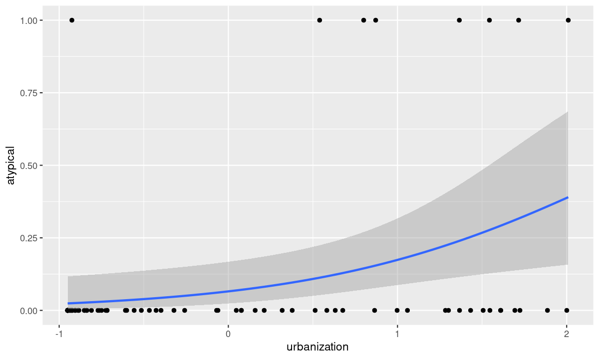

![:img right:0, bottom: 0, 65%, , ](figures/title-plot6-1.png)
![:img right: 1%, top: 1%, 25%, ,](figures/Screaming_b.jpg)

## NRI 7350
# Even more stats...

Generalized linear models,   
Other advanced models,   
Non-parametric stats

---
class: section

# Getting started (again)

Open RStudio  
Open your NRI project  
Open a **new** script for today:

File > New File > R Script

Make sure to load packages at the top:  
`library(tidyverse)`    
`library(DHARMa)`

---
class: section

# Reference Material

This lecture covers A HUGE subject area

It is not comprehensive

It is a place to start, with references to guide you later on

---
class: section

# Diagnostics for complex models

### Introducing DHARMa

[DHARMa Tutorial](https://cran.r-project.org/web/packages/DHARMa/vignettes/DHARMa.html)   
.small[(Many great examples of model checking)]

---
class: space-list
# DHARMa Package

### *Simulated* Residuals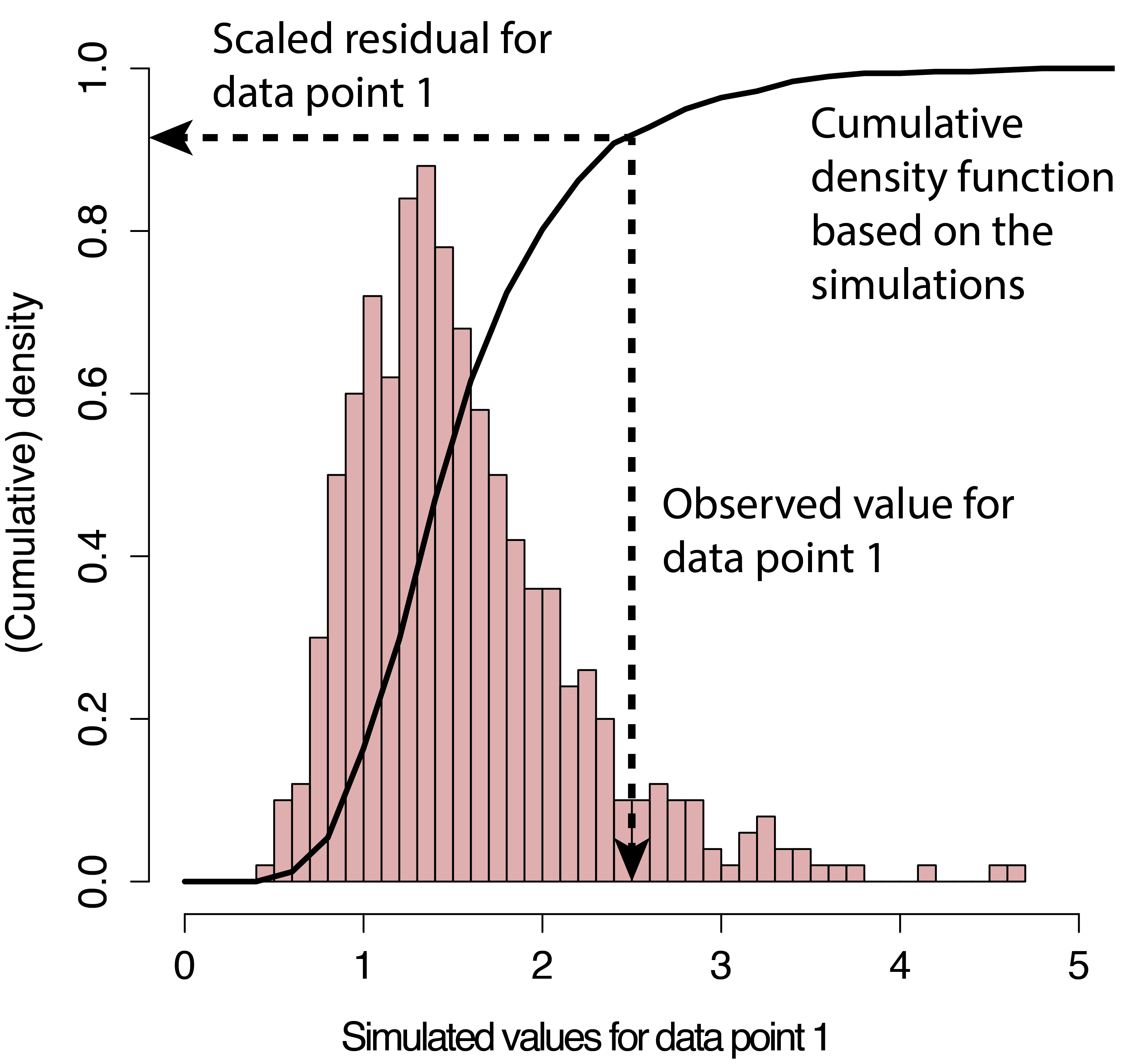

![:img right:15px, bottom: 0, 50%, Pink histogram showing simulated values for data point1 on the x-axis and cumulative density on the y](figures/DHARMa.png)

- **If** your data perfectly matched your model, what would the values look like? 
 - Pink histogram values show repeatedly simulated values
 
 
--

- How do your *actual* values compare? 
 - Black arrow on x-axis shows *actual* value
 - Black arrow on y-axis shows residual: 
 how *actual* value compares to distribution of simulated values

- Residuals are scaled (0 to 1)
  - If data fits model perfectly, expect all = 0.5
  - Good fit *always* = flat/uniform distribution

---
class: space-list
# DHARMa Package

### *If* data fits the model

![:spacer 20px]()

- Residuals follow a flat (uniform) distribution (no matter what model!)

- Expect: Straight line on QQ plot of **uniform** distribution .small[**(similar to QQ Normal plot)**]
- Expect: No patterns between residuals and model predictions .small[**(similar to heteroscedasticity plot, resid vs. fitted)**]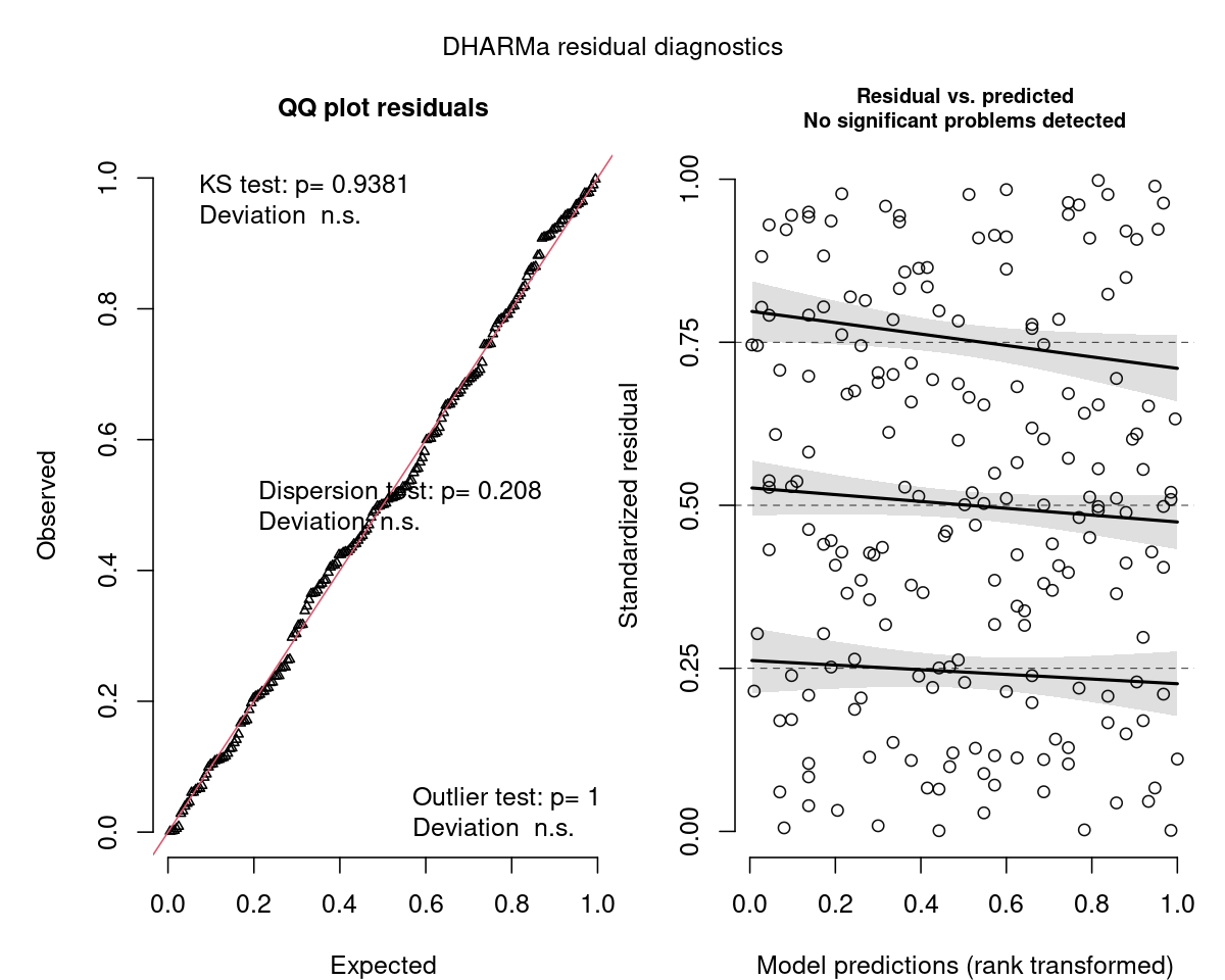

![:img right: 0, bottom: 5px, 59%, , ](./figures/dharma1-1.png)

![:box 50%, 40%, 70%](Note These aren't the same kinds of plots we did in the last couple of labs. BUT you can interpret them the same way, when looking for problems)

---
class: split-50
# DHARMa Package

.columnl[
### QQ Plot
.medium[
- Tests **Uniformity** with Kolmogorov-Smirnov (KS) test
  - (do the residuals match a Uniform distribution?)
- Tests for **Over/Underdispersion** with Dispersion Test
- Tests for more **Outliers** than expected with Outlier test
]

<img src="6 GLMs and Non-parametric stats - answers_files/figure-html/unnamed-chunk-1-1.png" width="100%" style="display: block; margin: auto;" />
]

.columnr[
### Residuals vs. Predicted

.medium[

- Check distribution of residuals .small[(visually and with quantiles)]
- Dotted lines show expected quantiles
- Black lines show simulated quantiles (want straight lines)
- Outliers would show up as red stars
]

]

---
# DHARMa Package

### Usage

```r
library(DHARMa)

m <- lm(body_mass_g ~ flipper_length_mm, data = penguins)
*r <- simulateResiduals(m, n = 1000, plot = TRUE)
```

- `simulateResiduals()` function from 
- Use `plot = TRUE` to produce diagnostic plots to see if simulated match expectation
- `n = 1000` isn't strictly necessary but runs more simulations to produce more stable results

--
### Applies to any model

- REMEMBER! Not assessing normality of residuals or heteroscedacity...
- Assessing whether data fits the model
- This *includes* assumptions, but *also* includes general fit, etc.
- So, we can use this to see if our model could be improved...

---
# DHARMa Package

### Check a previous model

```r
m <- lm(body_mass_g ~ flipper_length_mm, data = penguins)
r <- simulateResiduals(m, n = 1000, plot = TRUE)
```

![:box 50%, 50%, 40%](Remember how species and sex influenced body measurements?)

---
# DHARMa Package

### Improve the fit...

---
class: section

# Comparing Models

### Model Selection

---
# Model Selection

### How do I know which model to use?

1. Check your diagnostics
  - Generally speaking, pick the model which has good diagnostics
  
  .spacer[]

--
  
  **All models have reasonably good diagnostics?**
  
  .spacer[]
  
--

2. Check model fit (how good is model at explaining data?)
  - Analysis of Variance/Deviance - `anova()`
    
  - Information Theoretic Approach (AIC) - `model.sel()` (MuMIn package)
      -  (covered in class Nov 17th)

> Many other methods, functions, packages

---
# `anova()` - Analysis of Variance/Deviance

### Very common in R

- Sequential analysis of variance for `lm()`
- Analysis of deviance for `glm()`

```r
p <- na.omit(penguins) # Must have exact same dataset for each model

m1 <- lm(body_mass_g ~ flipper_length_mm, data = p)
m2 <- lm(body_mass_g ~ flipper_length_mm + species + sex, data = p)
m3 <- lm(body_mass_g ~ flipper_length_mm + species * sex, data = p)

anova(m1, m2, m3)
```

---
# `anova()` - Analysis of Variance/Deviance

```r
anova(m1, m2, m3)
```

```
## Analysis of Variance Table
## 
## Model 1: body_mass_g ~ flipper_length_mm
## Model 2: body_mass_g ~ flipper_length_mm + species + sex
## Model 3: body_mass_g ~ flipper_length_mm + species * sex
## Res.Df RSS Df Sum of Sq F Pr(>F) 
## 1 331 51211963 
## 2 328 28653568 3 22558395 91.082 < 2.2e-16 ***
## 3 326 26913579 2 1739989 10.538 3.675e-05 ***
## ---
## Signif. codes: 0 '***' 0.001 '**' 0.01 '*' 0.05 '.' 0.1 ' ' 1
```

---
# `anova()` - Analysis of Variance/Deviance

```r
anova(m1, m2, m3)
```

```
## Analysis of Variance Table
## 
*## Model 1: body_mass_g ~ flipper_length_mm
*## Model 2: body_mass_g ~ flipper_length_mm + species + sex
*## Model 3: body_mass_g ~ flipper_length_mm + species * sex
## Res.Df RSS Df Sum of Sq F Pr(>F) 
## 1 331 51211963 
## 2 328 28653568 3 22558395 91.082 < 2.2e-16 ***
## 3 326 26913579 2 1739989 10.538 3.675e-05 ***
## ---
## Signif. codes: 0 '***' 0.001 '**' 0.01 '*' 0.05 '.' 0.1 ' ' 1
```

- Models being compared

---
# `anova()` - Analysis of Variance/Deviance

```r
anova(m1, m2, m3)
```

```
## Analysis of Variance Table
## 
## Model 1: body_mass_g ~ flipper_length_mm
## Model 2: body_mass_g ~ flipper_length_mm + species + sex
## Model 3: body_mass_g ~ flipper_length_mm + species * sex
## Res.Df RSS Df Sum of Sq F Pr(>F) 
*## 1 331 51211963 
*## 2 328 28653568 3 22558395 91.082 < 2.2e-16 ***
*## 3 326 26913579 2 1739989 10.538 3.675e-05 ***
## ---
## Signif. codes: 0 '***' 0.001 '**' 0.01 '*' 0.05 '.' 0.1 ' ' 1
```

- Models being compared
- How the models compare

---
# `anova()` - Analysis of Variance/Deviance

```r
anova(m1, m2, m3)
```

```
## Analysis of Variance Table
## 
## Model 1: body_mass_g ~ flipper_length_mm
## Model 2: body_mass_g ~ flipper_length_mm + species + sex
## Model 3: body_mass_g ~ flipper_length_mm + species * sex
## Res.Df RSS Df Sum of Sq F Pr(>F) 
## 1 331 51211963 
*## 2 328 28653568 3 22558395 91.082 < 2.2e-16 ***
## 3 326 26913579 2 1739989 10.538 3.675e-05 ***
## ---
## Signif. codes: 0 '***' 0.001 '**' 0.01 '*' 0.05 '.' 0.1 ' ' 1
```

- Models being compared
- How the models compare
 - m2 has significantly (P < 0.05) lower Sums Squares than m1

---
# `anova()` - Analysis of Variance/Deviance

```r
anova(m1, m2, m3)
```

```
## Analysis of Variance Table
## 
## Model 1: body_mass_g ~ flipper_length_mm
## Model 2: body_mass_g ~ flipper_length_mm + species + sex
## Model 3: body_mass_g ~ flipper_length_mm + species * sex
## Res.Df RSS Df Sum of Sq F Pr(>F) 
## 1 331 51211963 
## 2 328 28653568 3 22558395 91.082 < 2.2e-16 ***
*## 3 326 26913579 2 1739989 10.538 3.675e-05 ***
## ---
## Signif. codes: 0 '***' 0.001 '**' 0.01 '*' 0.05 '.' 0.1 ' ' 1
```

- Models being compared
- How the models compare
 - m2 has significantly (P < 0.05) lower Sums Squares than m1
 - m3 has significantly (P < 0.05) lower Sums Squares than m2

![:box 25%, 50%, 25%](Therefore m3 > m2 > m1)

---
# `model.sel()` - AIC model selection

```r
library(MuMIn)
model.sel(m1, m2, m3)
```

```
## Model selection table 
##      (Int) flp_lng_mm sex spc sex:spc             family df    logLik   AICc  delta weight
## m3  -478.3      20.49   +   +       + gaussian(identity)  8 -2353.956 4724.4   0.00      1
## m2  -365.8      20.02   +   +         gaussian(identity)  6 -2364.387 4741.0  16.67      0
## m1 -5872.0      50.15                 gaussian(identity)  3 -2461.073 4928.2 203.86      0
## Models ranked by AICc(x)
```

- m3 is the best (lowest AICc, and much lower than the others)
- For more specifics on how to use/interpret this table, 
  stay tuned for Nicky's lecture

![:spacer 20px]()

> Always, remember that your 'best' model is only the best of what you've 
> compared...

---
class: section
# Generalized Linear Models

[Chapter 13, "The R Book" by Michael J. Crawley](https://search.lib.umanitoba.ca/permalink/01UMB_INST/k6qbb2/cdi_skillsoft_books24x7_bks00051275)  
.small[(Freely available online through University of Manitoba Library)]

---
# Generalized linear models

![:circle center, 50%, 150px, 150px, middle, lightblue, black](Simple Linear Models)

![:circle center, 50%, 150px, 150px, middle, lightblue, black](General Linear Models)

- Residuals are normally distributed
- Normally distributed also known as "Gaussian" distribution

![:circle center, 50%, 150px, 150px, middle, lightblue, black](Gaussian Family)

---
# Generalized linear models

- One type of Generalized linear model

![:circle 5.75%, 20%, 625px, 500px, top, cornflowerblue, white](<div style = "padding: 20px;"><large>Generalized Linear Models</large></div>)
![:circle center, 50%, 150px, 150px, middle, lightblue, black](Gaussian Family)

- So what if your residuals are *not* normal?
  - ie. they don't follow a Gaussian distribution  
  
  
--

- Try a different family!

![:circle 25.5%, 35%, 150px, 150px, middle, lightblue, black](Poisson Family)

![:circle 7%, 50%, 150px, 150px, middle, lightblue, black](Negative Binomial Family)

![:circle 25.5%, 70%, 150px, 150px, middle, lightblue, black](Binomial Family)

- Etc.

---
# Generalized linear models

### Gaussian Family .small[(Normal data)]

```r
lm(y ~ x1 * x2, data = my_data)
```

---
# Generalized linear models

### Poisson Family .small[(Count data)]

```r
glm(counts ~ x1 * x2, family = "poisson", data = my_data)
```

---
# Generalized linear models

### Negative Binomial Family .small[(Overdispersed Count data)]
.small[

```r
MASS::glm.nb(counts ~ x1 * x2,  data = my_data)
```
]

- Do Poisson model first
- Check diagnostics, if necessary, you'll do a negative binomial model

---
# Generalized linear models

### Binomial Family .small[(Binary data)]

- TRUE/FALSE, 0/1, Logistic Regression

```r
glm(y ~ x1 * x2, family = "binomial", data = my_data)
```

---
# Generalized linear models

### Binomial Family .small[(Binary data)]

- TRUE/FALSE, 0/1, Logistic Regression

```r
glm(y ~ x1 * x2, family = "binomial", data = my_data)
```

### Binomial Family .small[(Proportion data)]

- Two responses (binary outcomes), each in it's own column 
  - .medium[(e.g., number of Yes, vs. No; Number of songs, vs. calls)]

```r
glm(cbind(yes, no) ~ x1 * x2, family = "binomial", data = my_data)
```

---
class: section

# Examples

---
# Count Data - Poisson Family

### Get the data

```r
p <- read_csv("https://stats.idre.ucla.edu/stat/data/poisson_sim.csv")
p <- mutate(p, program = factor(prog, levels = 1:3,
 labels = c("General", "Academic", "Vocational")))
p
```

.small[

```
## # A tibble: 200 × 5
## id num_awards prog math program 
## <dbl> <dbl> <dbl> <dbl> <fct> 
## 1 45 0 3 41 Vocational
## 2 108 0 1 41 General 
## 3 15 0 3 44 Vocational
## 4 67 0 3 42 Vocational
## 5 153 0 3 40 Vocational
## 6 51 0 1 42 General 
## 7 164 0 3 46 Vocational
## 8 133 0 3 40 Vocational
## 9 2 0 3 33 Vocational
## 10 53 0 3 46 Vocational
## # … with 190 more rows
```

]

![:box 25%, 60%, 35%](How do marks in <code>math</code> as well as <code>program</code> of study influence the number of awards a student receives (<code>num_awards</code>&rpar;?)

---
# Count Data - Poisson Family

### Look at the data

```r
ggplot(data = p, aes(x = math, y = num_awards, colour = program)) +
  geom_point()
```

---
# Count Data - Poisson Family

### Look at the data

```r
ggplot(data = p, aes(x = math, y = num_awards, colour = program)) +
  geom_point() +
* stat_smooth(method = "glm", se = FALSE)
```

<img src="6 GLMs and Non-parametric stats - answers_files/figure-html/unnamed-chunk-26-1.png" width="70%" style="display: block; margin: auto;" />
---
# Count Data - Poisson Family

### Look at the data

```r
ggplot(data = p, aes(x = math, y = num_awards, colour = program)) +
  geom_point() +
* stat_smooth(method = "glm", method.args = list(family = "poisson"), se = FALSE)
```

---
class: split-60
# Count Data - Poisson Family

### Run the model

```r
m <- glm(num_awards ~ math + program, family = "poisson", data = p)
```

---
class: split-60
# Count Data - Poisson Family

.columnl[

### Diagnostics

```r
summary(m)
```

.small[

```
## Call:
## glm(formula = num_awards ~ math + program, family = "poisson", 
##     data = p)
## 
## Coefficients:
##                   Estimate Std. Error z value Pr(>|z|)    
## (Intercept)       -5.24712    0.65845  -7.969 1.60e-15 ***
## math               0.07015    0.01060   6.619 3.63e-11 ***
## programAcademic    1.08386    0.35825   3.025  0.00248 ** 
## programVocational  0.36981    0.44107   0.838  0.40179    
## ---
## Signif. codes:  0 '***' 0.001 '**' 0.01 '*' 0.05 '.' 0.1 ' ' 1
## 
*## (Dispersion parameter for poisson family taken to be 1)
## 
##     Null deviance: 287.67  on 199  degrees of freedom
## Residual deviance: 189.45  on 196  degrees of freedom
## AIC: 373.5
## 
## Number of Fisher Scoring iterations: 6
```

]

.columnr[
### Overdispersion

.medium[
- Dispersion = Residual Deviance / DF
- Expected to be 1 for Poisson
- Overdispersion > 1; Underdispersion < 1
]]

---
class: split-60
# Count Data - Poisson Family

.columnl[

### Diagnostics

```r
summary(m)
```

.small[

```
## Call:
## glm(formula = num_awards ~ math + program, family = "poisson", 
##     data = p)
## 
## Coefficients:
##                   Estimate Std. Error z value Pr(>|z|)    
## (Intercept)       -5.24712    0.65845  -7.969 1.60e-15 ***
## math               0.07015    0.01060   6.619 3.63e-11 ***
## programAcademic    1.08386    0.35825   3.025  0.00248 ** 
## programVocational  0.36981    0.44107   0.838  0.40179    
## ---
## Signif. codes:  0 '***' 0.001 '**' 0.01 '*' 0.05 '.' 0.1 ' ' 1
## 
## (Dispersion parameter for poisson family taken to be 1)
## 
##     Null deviance: 287.67  on 199  degrees of freedom
*## Residual deviance: 189.45  on 196  degrees of freedom
## AIC: 373.5
## 
## Number of Fisher Scoring iterations: 6
```

]

.columnr[
### Overdispersion

.medium[
- Dispersion = Residual Deviance / DF
- Expected to be 1 for Poisson
- Overdispersion > 1; Underdispersion < 1
]

.medium[
**Traditional check:**
- Residual Deviance (189.45) vs. DF (196)
]
.small[

```r
deviance(m) / df.residual(m)
```

```
## [1] 0.9665797
```
]

.medium[
- Almost 1 .small[(which it is good)]
]

.small[

```r
pchisq(deviance(m), df.residual(m), 
       lower.tail = FALSE)
```

```
## [1] 0.6182274
```
]
.medium[
- Test shows no significant overdispersion  
  (p = 0.62)
]]

---
class: split-50
# Count Data - Poisson Family

### Diagnostics

- Residuals are complicated to assess in GLMs
- Therefore, use `DHARMa` package!

```r
r <- simulateResiduals(m, n = 1000, plot = TRUE)
```

![:box 25%, 25%, 25%](Also shows no overdispersion (See Dispersion test&rpar;)

---
class: split-50
# Count Data - Poisson Family - Model Diagnostics

### Zero-inflation .small[(More zeros than expected)]

- Will often pop up as iffy residuals
- Overdispersion can lead to false positives
- Here not a problem (non-significant P-value)

```r
testZeroInflation(m, plot = FALSE)
```

```
## 
## 	DHARMa zero-inflation test via comparison to expected zeros with simulation under H0 =
## 	fitted model
## 
## data:  simulationOutput
## ratioObsSim = 1.0131, p-value = 0.832
## alternative hypothesis: two.sided
```

---
class: split-60, space-list
# Count Data - Poisson Family

.columnl[
### Interpretation

```r
summary(m)
```

.small[

```
## Call:
## glm(formula = num_awards ~ math + program, family = "poisson", 
##     data = p)
## 
## Coefficients:
##                   Estimate Std. Error z value Pr(>|z|)    
*## (Intercept)       -5.24712    0.65845  -7.969 1.60e-15 ***
*## math               0.07015    0.01060   6.619 3.63e-11 ***
*## programAcademic    1.08386    0.35825   3.025  0.00248 ** 
*## programVocational  0.36981    0.44107   0.838  0.40179    
## ---
## Signif. codes:  0 '***' 0.001 '**' 0.01 '*' 0.05 '.' 0.1 ' ' 1
## 
## (Dispersion parameter for poisson family taken to be 1)
## 
##     Null deviance: 287.67  on 199  degrees of freedom
## Residual deviance: 189.45  on 196  degrees of freedom
## AIC: 373.5
## 
## Number of Fisher Scoring iterations: 6
```

]
]

.columnr[
### Effects

.medium[
- Significantly more awards received with higher marks in math
  - i.e. Number of awards increases by 0.07 log-counts per 1 unit increase in Math mark
- Significantly more awards received in Academic Program compared to General
  - i.e. Number of awards greater by 1.08 log-counts for Academic compared to General
- No difference in amount of awards received in Vocational vs. General Program
]]

![:img right: 35px, bottom: 30px, 37%](figures/wtf_allison_horst.jpeg)

---
class: split-60, space-list
# Count Data - Poisson Family

.columnl[
### Interpretation

```r
summary(m)
```

.small[

]
]

.columnr[

### Interpreting Results
.medium[
- Convert to ratios with `\(e^{\textrm{est}}\)` (`exp()`)
]
.small[

```r
data.frame(est = coef(m), 
           ratios = exp(coef(m)))
```

```
##                          est     ratios
## (Intercept)       -5.2471244 0.00526263
## math               0.0701524 1.07267164
## programAcademic    1.0838591 2.95606545
## programVocational  0.3698092 1.44745846
```
]

.medium[
- No. awards increases by 1.07 *times* per 1 unit increase in Math mark (7%)
- No. awards received by Academic is 2.96 *times* greater than in General program
]]

---
# Overdispersion

.medium[
- Overdispersion when data is spread out more than distribution would be (longer tails)
- Results in **highly** significant findings that are **not** valid!!
- Simulated residuals run from 0 to 1, but here more residuals around 0 and 1 (longer tails)
]

---
# Underdispersion

.medium[
- Underdispersion is less common
- When data is gathered towards the centre more than distribution would be (shorter tails)
- These simulated residuals run from 0 to 1
- Here, more residuals around 0.5 (shorter tails)
]

---
class: split-50
# Overdispersed Count Data - Negative Binomial

```r
quine <- MASS::quine
```

.columnl[
### Poisson GLM
.medium[

<code class ='r hljs remark-code'>m1 <- glm(Days ~ Sex, data = quine, family = "poisson") summary(m1)</code>
]
.small[

```
## Coefficients:
## Estimate Std. Error z value Pr(>|z|) 
## (Intercept) 2.72294 0.02865 95.030 < 2e-16 ***
## SexM 0.16490 0.04080 4.041 5.31e-05 ***
## ---
## Signif. codes: 0 '***' 0.001 '**' 0.01 '*' 0.05 '.' 0.1 ' ' 1
## 
## (Dispersion parameter for poisson family taken to be 1)
## 
## Null deviance: 2073.5 on 145 degrees of freedom
## Residual deviance: 2057.2 on 144 degrees of freedom
```

]]

.columnr[
### Negative Binomial GLM
.medium[

<code class ='r hljs remark-code'>m2 <- MASS::glm.nb(Days ~ Sex, data = quine) summary(m2)</code>
]
.small[

```
## Coefficients:
## Estimate Std. Error z value Pr(>|z|) 
## (Intercept) 2.7229 0.1116 24.395 <2e-16 ***
## SexM 0.1649 0.1656 0.996 0.319 
## ---
## Signif. codes: 0 '***' 0.001 '**' 0.01 '*' 0.05 '.' 0.1 ' ' 1
## 
## (Dispersion parameter for Negative Binomial(1.0741) family taken to be 1)
## 
## Null deviance: 169.50 on 145 degrees of freedom
## Residual deviance: 168.51 on 144 degrees of freedom
```
]]

---
class: split-50
# Overdispersed Count Data - Negative Binomial

```r
quine <- MASS::quine
```

.columnl[
### Poisson GLM
.medium[

```
## Coefficients:
## Estimate Std. Error z value Pr(>|z|) 
## (Intercept) 2.72294 0.02865 95.030 < 2e-16 ***
*## SexM 0.16490 0.04080 4.041 5.31e-05 ***
## ---
## Signif. codes: 0 '***' 0.001 '**' 0.01 '*' 0.05 '.' 0.1 ' ' 1
## 
## (Dispersion parameter for poisson family taken to be 1)
## 
## Null deviance: 2073.5 on 145 degrees of freedom
*## Residual deviance: 2057.2 on 144 degrees of freedom
```

]]

.columnr[
### Negative Binomial GLM
.medium[

<code class ='r hljs remark-code'>m2 <- MASS::glm.nb(Days ~ Sex, data = quine) summary(m2)</code>
]
.small[

```
## Coefficients:
## Estimate Std. Error z value Pr(>|z|) 
## (Intercept) 2.7229 0.1116 24.395 <2e-16 ***
*## SexM 0.1649 0.1656 0.996 0.319 
## ---
## Signif. codes: 0 '***' 0.001 '**' 0.01 '*' 0.05 '.' 0.1 ' ' 1
## 
## (Dispersion parameter for Negative Binomial(1.0741) family taken to be 1)
## 
## Null deviance: 169.50 on 145 degrees of freedom
*## Residual deviance: 168.51 on 144 degrees of freedom
```
]]

---
class: split-50
# Overdispersed Count Data - Negative Binomial

.columnl[
### Poisson GLM

```r
r <- simulateResiduals(m1)
plotQQunif(r) # Just the first Uniformity Plot
```

<img src="6 GLMs and Non-parametric stats - answers_files/figure-html/unnamed-chunk-51-1.png" width="100%" style="display: block; margin: auto;" />
]

.columnr[
### Negative Binomial GLM

```r
r <- simulateResiduals(m2)
plotQQunif(r) # Just the first Uniformity Plot
```

<img src="6 GLMs and Non-parametric stats - answers_files/figure-html/unnamed-chunk-52-1.png" width="100%" style="display: block; margin: auto;" />
]

![:box 50%, 80%, 45%](Negative Binomial is definitely a better fit Good thing we checked!)

---
# Binary Data (0/1) - Binomial Family .small[(logistic regresion)]

### Get the data

- Mountain chickadees atypical songs by urbanization
- Negative `urbanization` more rural
- Positive `urbanization` more urban 
- `atypical_c` atypical singer (1) or 'normal' singer (0)

```r
atypical <- read_csv("https://steffilazerte.ca/NRI_7350/data/atypical.csv")
atypical
```

```
## # A tibble: 78 × 2
## atypical urbanization
## <dbl> <dbl>
## 1 1 0.540
## 2 0 0.582
## 3 0 -0.950
## 4 0 -0.950
## 5 0 0.513
## 6 0 1.69 
## 7 0 1.51 
## 8 0 1.72 
## 9 0 1.28 
## 10 0 1.43 
## # … with 68 more rows
```

![:img right:25px, top:15%, 29%, Ken Otter,](figures/Screaming_b.jpg)

---
# Binary Data (0/1) - Binomial Family .small[(logistic regresion)]

### Look at the data

```r
ggplot(data = atypical, aes(x = urbanization, y = atypical)) +
  geom_point() +
  stat_smooth(method = "glm", method.args = list(family = "binomial"))
```

![:img right:25px, top:15%, 23%, Ken Otter,](figures/Screaming_b.jpg)

---
# Binary Data (0/1) - Binomial Family .small[(logistic regresion)]

### Run model and check diagnostics
.small[

```r
m <- glm(atypical ~ urbanization, family = "binomial", data = atypical)
r <- simulateResiduals(m, plot = TRUE)
```

<img src="6 GLMs and Non-parametric stats - answers_files/figure-html/unnamed-chunk-56-1.png" width="100%" style="display: block; margin: auto;" />
]

![:img right:25px, top:15%, 23%, Ken Otter,](figures/Screaming_b.jpg)

---
class: split-60
# Binary Data (0/1) - Binomial Family .small[(logistic regresion)]

.columnl[

```r
summary(m)
```

.small[

```
## 
## Call:
## glm(formula = atypical ~ urbanization, family = "binomial", data = atypical)
## 
## Deviance Residuals: 
##     Min       1Q   Median       3Q      Max  
## -0.9907  -0.4460  -0.2500  -0.2210   2.7201  
## 
## Coefficients:
##              Estimate Std. Error z value Pr(>|z|)    
## (Intercept)   -2.6572     0.5380  -4.939 7.85e-07 ***
## urbanization   1.1000     0.4209   2.613  0.00897 ** 
## ---
## Signif. codes:  0 '***' 0.001 '**' 0.01 '*' 0.05 '.' 0.1 ' ' 1
## 
## (Dispersion parameter for binomial family taken to be 1)
## 
##     Null deviance: 51.586  on 77  degrees of freedom
## Residual deviance: 43.203  on 76  degrees of freedom
## AIC: 47.203
## 
## Number of Fisher Scoring iterations: 6
```

]
]

.columnr[
### Interpreting Results

```r
exp(coef(m))
```

```
##  (Intercept) urbanization 
##   0.07014254   3.00406665
```

.medium[
E.g., The odds of being an atypical singer increase by a factor of 3 (x3 times more likely) for every unit increase in Habit Urbanization.
]]

![:img right:11%, bottom:10%, 23%, Ken Otter,](figures/Screaming_b.jpg)

---
# Binary Outcomes - Binomial Family

Proportion with binary outcomes (e.g., 10 yes, 5 no)

### Get the data

```r
admissions <- as.data.frame(UCBAdmissions)
admissions <- pivot_wider(admissions, 
 names_from = Admit, 
 values_from = Freq) 
admissions
```

```
## # A tibble: 12 × 4
## Gender Dept Admitted Rejected
## <fct> <fct> <dbl> <dbl>
## 1 Male A 512 313
## 2 Female A 89 19
## 3 Male B 353 207
## 4 Female B 17 8
## 5 Male C 120 205
## 6 Female C 202 391
## 7 Male D 138 279
## 8 Female D 131 244
## 9 Male E 53 138
## 10 Female E 94 299
## 11 Male F 22 351
## 12 Female F 24 317
```

---
class: split-60
# Binary Outcomes - Binomial Family

.columnl[
### Diagnostics

```r
m <- glm(cbind(Admitted, Rejected) ~ Gender, 
 family = "binomial", data = admissions)
summary(m)
```

.small[

```
## Call:
## glm(formula = cbind(Admitted, Rejected) ~ Gender, family = "binomial", 
## data = admissions)
## 
## Coefficients:
## Estimate Std. Error z value Pr(>|z|) 
## (Intercept) -0.22013 0.03879 -5.675 1.38e-08 ***
## GenderFemale -0.61035 0.06389 -9.553 < 2e-16 ***
## ---
## Signif. codes: 0 '***' 0.001 '**' 0.01 '*' 0.05 '.' 0.1 ' ' 1
## 
## (Dispersion parameter for binomial family taken to be 1)
## 
*## Null deviance: 877.06 on 11 degrees of freedom
## Residual deviance: 783.61 on 10 degrees of freedom
## AIC: 856.55
## 
## Number of Fisher Scoring iterations: 4
```

]
]

.columnr[

### Overdispersion

.medium[
**Traditional check:**
- Look at resid deviance (783.61) vs. df (10)
]

.small[

```r
deviance(m) / df.residual(m)
```

```
## [1] 78.3607
```
]

.medium[
- Very large .small[(definitely not close to 1)]
]

.small[

```r
pchisq(deviance(m), df.residual(m), 
       lower.tail = FALSE)
```

```
## [1] 6.892992e-162
```
]
.medium[
- Test shows significant overdispersion
]]

---
# Binary Outcomes - Binomial Family

### Check with DHARMa

```r
plotQQunif(m)
plotResiduals(m, asFactor = TRUE) # to ensure Gender is treated as category
```

![:box 50%, 85%, 30%](Okay, how do we deal with this?)

---
# Binary Outcomes - Quasi-binomial Family .small[for overdispersion]

```r
m_quasi <- glm(cbind(Admitted, Rejected) ~ Gender, family = "quasibinomial", data = admissions)
summary(m_quasi)
```

.small[

```
## 
## Call:
## glm(formula = cbind(Admitted, Rejected) ~ Gender, family = "quasibinomial", 
##     data = admissions)
## 
## Deviance Residuals: 
##      Min        1Q    Median        3Q       Max  
## -16.7915   -4.7613   -0.4365    5.1025   11.2022  
## 
## Coefficients:
##              Estimate Std. Error t value Pr(>|t|)
## (Intercept)   -0.2201     0.3281  -0.671    0.517
## GenderFemale  -0.6104     0.5404  -1.129    0.285
## 
*## (Dispersion parameter for quasibinomial family taken to be 71.52958)
## 
##     Null deviance: 877.06  on 11  degrees of freedom
## Residual deviance: 783.61  on 10  degrees of freedom
## AIC: NA
## 
## Number of Fisher Scoring iterations: 4
```

]

![:box 25%, 50%, 35%](Much more appropriate But 'quasi' families don't always work with other functions/packages, like DHARMa!)

---
# Binary Outcomes - Mixed models .small[for overdispersion]

- Observation-level random effects (i.e assign each observation an ID number)

```r
library(lme4)
admissions <- mutate(admissions, ID = 1:n())
m_glmm <- glmer(cbind(Admitted, Rejected) ~ Gender + (1|ID), family = "binomial", data = admissions)
```

---
class: split-50
# Binary Outcomes - Overdispersion

Either way, fixing overdispersion remove the 'significance'

### Original

```r
coef(summary(m))
```

.small[

```
##                Estimate Std. Error   z value     Pr(>|z|)
## (Intercept)  -0.2201340 0.03878810 -5.675297 1.384479e-08
*## GenderFemale -0.6103524 0.06389305 -9.552720 1.263352e-21
```

]

![:spacer 10px]()

.columnl[
### Quasi fix

```r
coef(summary(m_quasi))
```

.small[

```
##                Estimate Std. Error    t value  Pr(>|t|)
## (Intercept)  -0.2201340  0.3280510 -0.6710359 0.5173966
*## GenderFemale -0.6103524  0.5403765 -1.1294947 0.2850545
```

]
]

.columnr[
### GLMM fix

```r
coef(summary(m_glmm))
```

.small[

```
##                Estimate Std. Error   z value  Pr(>|z|)
## (Intercept)  -0.6508845  0.4932596 -1.319558 0.1869827
*## GenderFemale  0.1747094  0.7016048  0.249014 0.8033499
```

]
]

---
class: split-30
# Your Turn!

.columnl[
We have the `crabs` dataset
]
.columnr[

```r
crabs <- read_csv("https://steffilazerte.ca/NRI_7350/data/crabs.csv")
```
]

![:spacer 20px]()

### Background

- Horseshoe crabs form pairs for spawning (mating)
- But extra, unattached males crowd around and try to get involved (Satellite males)

### Your Job
You're interested in the effect of female size (`width`) on the number of male `satellites`

- Look at your data (make a plot)
- Run a `glm()` for count data
- Check your diagnostics. Do you have a problem? Check for overdispersion and zero-inflation
- Apply an overdispersion fix
- Check your diagnostics. Do you have a problem? Check for zero-inflation

![:img right: 5%, top:27%, 10%, , ](figures/horseshoe_crab.png)

.footnote[Brockmann HJ (1996). “Satellite Male Groups in Horseshoe Crabs, *Limulus polyphemus*”, Ethology, 102(1), 1–21.]

---
exclude: FALSE
# Your Turn!

![:img right: 5px, top:20%, 10%, , ](figures/horseshoe_crab.png)

### Look at your data

```r
ggplot(data = crabs, aes(x = weight, y = satellites)) +
  geom_point() +
  stat_smooth(method = "glm", method.args = list(family = "poisson"))
```

---
exclude: FALSE
# Your Turn!

![:img right: 5px, top:20%, 10%, , ](figures/horseshoe_crab.png)

### Run a `glm()` for count data

.small[

```r
m <- glm(satellites ~ weight, data = crabs, family = "poisson")
summary(m)
```

```
## 
## Call:
## glm(formula = satellites ~ weight, family = "poisson", data = crabs)
## 
## Deviance Residuals: 
## Min 1Q Median 3Q Max 
## -2.9306 -1.9981 -0.5627 0.9299 4.9992 
## 
## Coefficients:
## Estimate Std. Error z value Pr(>|z|) 
## (Intercept) -0.4282 0.1789 -2.394 0.0167 * 
## weight 0.5892 0.0650 9.065 <2e-16 ***
## ---
## Signif. codes: 0 '***' 0.001 '**' 0.01 '*' 0.05 '.' 0.1 ' ' 1
## 
## (Dispersion parameter for poisson family taken to be 1)
## 
## Null deviance: 632.79 on 172 degrees of freedom
## Residual deviance: 560.84 on 171 degrees of freedom
## AIC: 920.14
## 
## Number of Fisher Scoring iterations: 5
```
]

---
exclude: FALSE
# Your Turn!

![:img right: 5px, top:20%, 10%, , ](figures/horseshoe_crab.png)

### Check your diagnostics
- Do you have a problem? Check for overdispersion and zero-inflation

```r
r <- simulateResiduals(m, plot = TRUE)
```

---
class: split-50
exclude: FALSE
# Your Turn!

![:img right: 5px, top:20%, 10%, , ](figures/horseshoe_crab.png)

### Check your diagnostics
- Do you have a problem? Check for overdispersion and zero-inflation

```r
testZeroInflation(m)
```

.columnl[
.small[

```
## 
## 	DHARMa zero-inflation test via comparison to expected zeros with simulation under H0 =
## 	fitted model
## 
## data: simulationOutput
## ratioObsSim = 4.381, p-value < 2.2e-16
## alternative hypothesis: two.sided
```
]]

.columnr[
<img src="6 GLMs and Non-parametric stats - answers_files/figure-html/unnamed-chunk-77-1.png" width="100%" style="display: block; margin: auto;" />
]

---
exclude: FALSE
# Your Turn!

![:img right: 5px, top:20%, 10%, , ](figures/horseshoe_crab.png)

### Apply an overdispersion fix

.small[

```r
m <- MASS::glm.nb(satellites ~ weight, data = crabs)
summary(m)
```

```
## 
## Call:
## MASS::glm.nb(formula = satellites ~ weight, data = crabs, init.theta = 0.9310998551, 
##     link = log)
## 
## Deviance Residuals: 
##     Min       1Q   Median       3Q      Max  
## -1.8393  -1.4123  -0.3246   0.4747   2.1278  
## 
## Coefficients:
##             Estimate Std. Error z value Pr(>|z|)    
## (Intercept)  -0.8637     0.4046  -2.135   0.0328 *  
## weight        0.7599     0.1578   4.817 1.46e-06 ***
## ---
## Signif. codes:  0 '***' 0.001 '**' 0.01 '*' 0.05 '.' 0.1 ' ' 1
## 
## (Dispersion parameter for Negative Binomial(0.9311) family taken to be 1)
## 
##     Null deviance: 216.44  on 172  degrees of freedom
## Residual deviance: 196.16  on 171  degrees of freedom
## AIC: 754.64
## 
## Number of Fisher Scoring iterations: 1
## 
## 
##               Theta:  0.931 
##           Std. Err.:  0.168 
## 
##  2 x log-likelihood:  -748.643
```
]

---
exclude: FALSE
# Your Turn!

![:img right: 5px, top:20%, 10%, , ](figures/horseshoe_crab.png)

### Check your diagnostics
- Do you still have a problem? Check for overdispersion and zero-inflation

```r
r <- simulateResiduals(m, plot = TRUE)
```

---
class: split-50
exclude: FALSE
# Your Turn!

![:img right: 5px, top:20%, 10%, , ](figures/horseshoe_crab.png)

### Check your diagnostics
- Do you still have a problem? Check for overdispersion and zero-inflation

```r
testZeroInflation(m)
```

.columnl[
.small[

```
## 
## 	DHARMa zero-inflation test via comparison to expected zeros with simulation under H0 =
## 	fitted model
## 
## data:  simulationOutput
## ratioObsSim = 1.2358, p-value = 0.088
## alternative hypothesis: two.sided
```
]]

.columnr[
<img src="6 GLMs and Non-parametric stats - answers_files/figure-html/unnamed-chunk-81-1.png" width="100%" style="display: block; margin: auto;" />
]

![:box 75%, 75%, 30%](Not bad... Can we do better?)

---
# Zero-inflated Models .small[(Advanced example! Above and beyond!)]

![:img right: 5px, top:100px, 10%, , ](figures/horseshoe_crab.png)

- `glmmTMB()` function from `glmmTMB` package
- Allows modeling zero-inflation (`ziformula` says zeros are a function of the variable `weight`)

.small[

```r
crabs <- read_csv("https://steffilazerte.ca/NRI_7350/data/crabs.csv")
library(glmmTMB)
m <- glmmTMB(satellites ~ weight, ziformula = ~ weight , family = "nbinom2", data = crabs)
summary(m)
```

```
## Dispersion parameter for nbinom2 family (): 4.96 
## 
## Conditional model:
##             Estimate Std. Error z value Pr(>|z|)   
## (Intercept)   0.8979     0.3051   2.943  0.00325 **
## weight        0.2171     0.1118   1.942  0.05217 . 
## ---
## Signif. codes:  0 '***' 0.001 '**' 0.01 '*' 0.05 '.' 0.1 ' ' 1
## 
## Zero-inflation model:
##             Estimate Std. Error z value Pr(>|z|)    
## (Intercept)   3.7546     0.9837   3.817 0.000135 ***
## weight       -1.9123     0.4320  -4.426 9.59e-06 ***
## ---
## Signif. codes:  0 '***' 0.001 '**' 0.01 '*' 0.05 '.' 0.1 ' ' 1
```
]

---
# Zero-inflated Models .small[(Advanced example! Above and beyond!)]

![:img right: 5px, top:100px, 10%, , ](figures/horseshoe_crab.png)

- `glmmTMB()` function from `glmmTMB` package
- Allows modeling zero-inflation (`ziformula` says zeros are a function of the variable `weight`)

.small[

```r
crabs <- read_csv("https://steffilazerte.ca/NRI_7350/data/crabs.csv")
library(glmmTMB)
m <- glmmTMB(satellites ~ weight, ziformula = ~ weight , family = "nbinom2", data = crabs)
summary(m)
```

```
## Dispersion parameter for nbinom2 family (): 4.96 
## 
*## Conditional model:
*##             Estimate Std. Error z value Pr(>|z|)   
*## (Intercept)   0.8979     0.3051   2.943  0.00325 **
*## weight        0.2171     0.1118   1.942  0.05217 . 
## ---
## Signif. codes:  0 '***' 0.001 '**' 0.01 '*' 0.05 '.' 0.1 ' ' 1
## 
## Zero-inflation model:
##             Estimate Std. Error z value Pr(>|z|)    
## (Intercept)   3.7546     0.9837   3.817 0.000135 ***
## weight       -1.9123     0.4320  -4.426 9.59e-06 ***
## ---
## Signif. codes:  0 '***' 0.001 '**' 0.01 '*' 0.05 '.' 0.1 ' ' 1
```
]

![:box 30%, 75%, 40%]("Regular" effects Heavier females have more satellite males (P = 0.052&rpar;)

---
# Zero-inflated Models .small[(Advanced example! Above and beyond!)]

![:img right: 5px, top:100px, 10%, , ](figures/horseshoe_crab.png)

- `glmmTMB()` function from `glmmTMB` package
- Allows modeling zero-inflation (`ziformula` says zeros are a function of the variable `weight`)

.small[

```r
crabs <- read_csv("https://steffilazerte.ca/NRI_7350/data/crabs.csv")
library(glmmTMB)
m <- glmmTMB(satellites ~ weight, ziformula = ~ weight , family = "nbinom2", data = crabs)
summary(m)
```

```
## Dispersion parameter for nbinom2 family (): 4.96 
## 
## Conditional model:
##             Estimate Std. Error z value Pr(>|z|)   
## (Intercept)   0.8979     0.3051   2.943  0.00325 **
## weight        0.2171     0.1118   1.942  0.05217 . 
## ---
## Signif. codes:  0 '***' 0.001 '**' 0.01 '*' 0.05 '.' 0.1 ' ' 1
## 
*## Zero-inflation model:
*##             Estimate Std. Error z value Pr(>|z|)    
*## (Intercept)   3.7546     0.9837   3.817 0.000135 ***
*## weight       -1.9123     0.4320  -4.426 9.59e-06 ***
## ---
## Signif. codes:  0 '***' 0.001 '**' 0.01 '*' 0.05 '.' 0.1 ' ' 1
```
]

![:box 30%, 75%, 40%]("Zero-inflation" effects more zeros counts as weight decreases What we expected!)

---
# Zero-inflated Models .small[(Advanced example! Above and beyond!)]

```r
r <- simulateResiduals(m, plot = TRUE)
```

![:img right: 5px, top:100px, 10%, , ](figures/horseshoe_crab.png)

.footnote[For more information on the glmmTMB package see their [Journal Article](https://journal.r-project.org/archive/2017/RJ-2017-066/RJ-2017-066.pdf)]

---
class: split-50
# Zero-inflated Models .small[(Advanced example! Above and beyond!)]

![:img right: 5px, top:100px, 10%, , ](figures/horseshoe_crab.png)

.footnote[For more information on the glmmTMB package see their [Journal Article](https://journal.r-project.org/archive/2017/RJ-2017-066/RJ-2017-066.pdf)]

```r
testZeroInflation(m)
```

.columnl[
.small[

```
## 
## 	DHARMa zero-inflation test via comparison to expected zeros with simulation under H0 =
## 	fitted model
## 
## data:  simulationOutput
## ratioObsSim = 1.0016, p-value = 1
## alternative hypothesis: two.sided
```
]]

.columnr[
<img src="6 GLMs and Non-parametric stats - answers_files/figure-html/unnamed-chunk-90-1.png" width="100%" style="display: block; margin: auto;" />
]

---
class: section

# Packages and References for Other Advanced Models

---
# Packages and References

### (Generalized) Linear Mixed Models (LMM, GLMM)
- Also called generalized linear mixed effects models (GLME, LME)
- `lme4` - More advanced, crossed-random factors, Generalized (`glmer()`) and Gaussian (`lmer()`)
- `nlme` - Older but can specify auto-correlation structures, only Gaussian (`lme()`)
- `glmmTMB` - Zero-inflated models and other distribtions

**References**

- [Ben Bolker's GLMM FAQ](https://bbolker.github.io/mixedmodels-misc/glmmFAQ.html)
- [Chapter 19, "The R Book" by Michael J. Crawley](https://search.lib.umanitoba.ca/permalink/01UMB_INST/k6qbb2/cdi_skillsoft_books24x7_bks00051275)  
.small[(Freely available online through University of Manitoba Library)]
- [Mixed Effects Models and Extensions in Ecology with R by Alain Zuur](https://search.lib.umanitoba.ca/permalink/01UMB_INST/1p55dqn/alma99149017057101651)    
.small[(Freely available online through University of Manitoba Library)]
- [Generalized linear mixed models: a practical guide for ecology and evolution](https://search.lib.umanitoba.ca/permalink/01UMB_INST/k6qbb2/cdi_proquest_miscellaneous_66983023), 2009, Trends in ecology and evolution

---
# Packages and References

### General Additive Models (GAM)
- `mgcv` package (`gam()`, `gamm()`)
- `gamm4` package (`gamm4()`)

**References**

- [Chapter 19, "The R Book" by Michael J. Crawley](https://search.lib.umanitoba.ca/permalink/01UMB_INST/k6qbb2/cdi_skillsoft_books24x7_bks00051275)  
.small[(Freely available online through University of Manitoba Library)]
- "Generalized Additive Models: An Introduction with R" by Simon N. Wood   
.small[(Hard-copy available from University of Manitoba Library)]

---
# Packages and References

### Generalized Estimating Equations (GEE)
- `gee` package (`gee()`)
- `geepack` package (`geeglm()`)

**References**

- [The R package geepack for Generalized Estimating equations](https://www.jstatsoft.org/article/view/v015i02), Journal of Statistical Software, 2005
- [geepack Manual](https://cran.r-project.org/web/packages/geepack/vignettes/geepack-manual.pdf)

---
class: section

# Non-parametric Statistics

---
# Non-parametric Statistics

### Wilcoxon Rank Sum (Mann-Whitney) Test

```r
air <- filter(airquality, Month %in% c(5, 8))
```

Is there a difference in air quality between May (5th month) and August (8th month)?

```r
wilcox.test(Ozone ~ Month, data = air, exact = FALSE)
```

```
## 
## 	Wilcoxon rank sum test with continuity correction
## 
## data:  Ozone by Month
## W = 127.5, p-value = 0.0001208
## alternative hypothesis: true location shift is not equal to 0
```

Yes!

---
# Non-parametric Statistics

### Kruskal-Wallis Rank Sum Test

Is there a difference in air quality among months?

```r
kruskal.test(Ozone ~ Month, data = airquality)
```

```
## 
## 	Kruskal-Wallis rank sum test
## 
## data:  Ozone by Month
## Kruskal-Wallis chi-squared = 29.267, df = 4, p-value = 6.901e-06
```

Yes, there is at least one month that is different from the rest.