library(bbsBayes)
#> bbsBayes v3.0.0
#> Note: version 3+ represents a major shift in functionality, noteably:
#>  - The Bayesian modelling engine has switched from *JAGS* to *Stan*
#>  - The workflow has been streamlined, resulting in deprecated/renamed
#>    function arguments
#> See the documentation for more details: https://BrandonEdwards.github.io/bbsBayes
library(ggplot2)
First make sure you have the BBS data downloaded
have_bbs_data()
#> Expected BBS state data 2022: '/home/runner/.local/share/R/bbsBayes/bbs_state_data_2022.rds'
#> [1] TRUE
If not, install with fetch_bbs_data()
Let’s start by running a quick (and dirty) model looking at the Pacific Wren.
m <- stratify(by = "bbs_cws", sample_data = TRUE) %>%
  prepare_data() %>%
  prepare_model(model = "first_diff") %>%
  run_model(iter_sampling = 20, iter_warmup = 20, chains = 2)
Or we can use the example model included in bbsBayes,
pacific_wren_model
m <- pacific_wren_modelNow we can calculate our convergence metrics
conv <- get_convergence(m)
conv
#> # A tibble: 10,495 × 5
#>    variable_type variable       rhat ess_bulk ess_tail
#>    <chr>         <chr>         <dbl>    <dbl>    <dbl>
#>  1 lp__          lp__          1.03      21.9     49.6
#>  2 strata_raw    strata_raw[1] 1.01      64.1     56.9
#>  3 strata_raw    strata_raw[2] 1.01      64.1     17.3
#>  4 strata_raw    strata_raw[3] 0.987     43.2     22.4
#>  5 strata_raw    strata_raw[4] 1.05      31.2     56.9
#>  6 strata_raw    strata_raw[5] 0.959     64.1     49.6
#>  7 strata_raw    strata_raw[6] 1.02      49.0     43.9
#>  8 strata_raw    strata_raw[7] 0.978     64.1     56.9
#>  9 strata_raw    strata_raw[8] 1.08      63.6     23.5
#> 10 strata_raw    strata_raw[9] 1.00      64.1     49.6
#> # … with 10,485 more rows
Wow, there are a lot of variables here.
We can visualize this by transforming the data frame and using ggplot2
tconv <- tidyr::pivot_longer(conv, cols = c(ess_bulk, ess_tail, rhat))

ggplot(data = tconv, aes(x = variable, y = value, colour = variable_type)) +
    geom_point() +
    facet_wrap(~name, scales = "free_y") +
    scale_colour_viridis_d(guide = FALSE)
#> Warning: Removed 123 rows containing missing values (`geom_point()`).
#> Warning: The `guide` argument in `scale_*()` cannot be `FALSE`. This was deprecated in
#> ggplot2 3.3.4.
#> ℹ Please use "none" instead.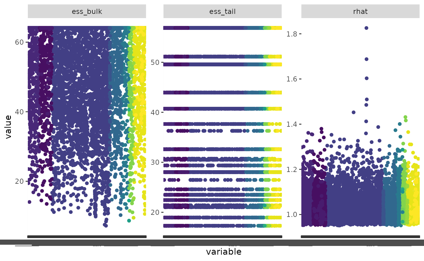
We can also choose to extract only some variables. To see which ones
are available, use the get_model_vars() function.
get_model_vars(m)
#>  [1] "lp__"          "strata_raw"    "STRATA"        "eta"
#>  [5] "obs_raw"       "ste_raw"       "sdnoise"       "sdobs"
#>  [9] "sdste"         "sdstrata"      "nu"            "sdbeta"
#> [13] "sdBETA"        "BETA_raw"      "beta_raw"      "E"
#> [17] "beta"          "yeareffect"    "BETA"          "YearEffect"
#> [21] "strata"        "phi"           "n"             "retrans_noise"
#> [25] "retrans_obs"   "retrans_ste"   "Hyper_N"       "adj"
We can also extract summary information from the model via the helper
function get_summary() (wrapper for
cmdstanr::summary())
get_summary(m)
#> # A tibble: 10,495 × 10
#> variable mean median sd mad q5 q95 rhat ess_b…¹
#> <chr> <dbl> <dbl> <dbl> <dbl> <dbl> <dbl> <dbl> <dbl>
#> 1 lp__ -1.38e+4 -1.38e+4 38.9 42.2 -1.38e+4 -1.37e+4 1.03 21.9
#> 2 strata_raw[1] -9.99e-1 -1.05e+0 0.351 0.396 -1.51e+0 -4.82e-1 1.01 64.1
#> 3 strata_raw[2] -1.99e-1 -1.63e-1 0.205 0.225 -4.86e-1 4.95e-2 1.01 64.1
#> 4 strata_raw[3] -1.36e-1 -6.58e-2 0.543 0.602 -1.06e+0 6.97e-1 0.987 43.2
#> 5 strata_raw[4] 1.57e+0 1.57e+0 0.267 0.221 1.03e+0 2.00e+0 1.05 31.2
#> 6 strata_raw[5] -1.48e-1 -1.11e-1 0.260 0.287 -5.78e-1 2.22e-1 0.959 64.1
#> 7 strata_raw[6] 1.26e+0 1.31e+0 0.638 0.717 6.03e-2 2.41e+0 1.02 49.0
#> 8 strata_raw[7] -1.12e+0 -1.22e+0 0.456 0.346 -1.64e+0 -3.86e-1 0.978 64.1
#> 9 strata_raw[8] 1.89e+0 1.94e+0 0.355 0.302 1.12e+0 2.35e+0 1.08 63.6
#> 10 strata_raw[9] -8.93e-1 -9.04e-1 0.258 0.263 -1.24e+0 -4.50e-1 1.00 64.1
#> # … with 10,485 more rows, 1 more variable: ess_tail <dbl>, and abbreviated
#> # variable name ¹ess_bulk