Create geofacet plot of population trajectories by province/state
Source:R/plot-geofacet.R
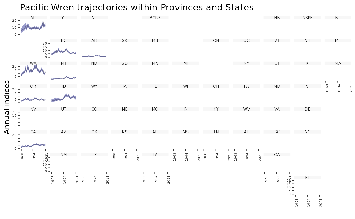
plot_geofacet.RdGenerate a faceted plot of population trajectories for each strata by
province/state. Given a model stratified by "state", "bbs_cws", or "bbs_usgs"
and indices generated by generate_indices() this function will generate a
faceted plot showing the population trajectories. All geofacet plots have one
facet per state/province, so if strata-level indices from the "bbs_cws" or
"bbs_usgs" are given, the function plots multiple trajectories (one for each
of the relevant strata) within each facet.
Usage
plot_geofacet(
  indices,
  ci_width = 0.95,
  multiple = FALSE,
  trends = NULL,
  slope = FALSE,
  add_observed_means = FALSE,
  col_viridis = FALSE,
  indices_list,
  stratify_by,
  species,
  select
)
Arguments
- indices
List. Indices generated by
generate_indices().- ci_width
quantile to define the width of the plotted credible interval. Defaults to 0.95, lower = 0.025 and upper = 0.975
- multiple
Logical, if TRUE, multiple strata-level trajectories are plotted within each prov/state facet
- trends
List. (Optional) Output generated by
generate_trends(). If included trajectories are coloured based on the same colour scale used inplot_map- slope
Logical. If dataframe of trends is included, whether colours in the plot should be based on slope trends. Default = FALSE
- add_observed_means
Should the facet plots include points indicating the observed mean counts. Defaults to FALSE. Note: scale of observed means and annual indices may not match due to imbalanced sampling among strata
- col_viridis
Logical flag to use "viridis" colour-blind friendly palette. Default is
FALSE- indices_list
Deprecated. Use
indicesinstead- stratify_by
Defunct.
- species
Defunct.
- select
Defunct.
Examples
# Using the example model for Pacific Wrens...
# Generate indices
i <- generate_indices(pacific_wren_model,
regions = c("stratum", "prov_state"))
#> Processing region stratum
#> Processing region prov_state
# Generate trends
t <- generate_trends(i)
# Now make the geofacet plot.
plot_geofacet(i, trends = t, multiple = TRUE)
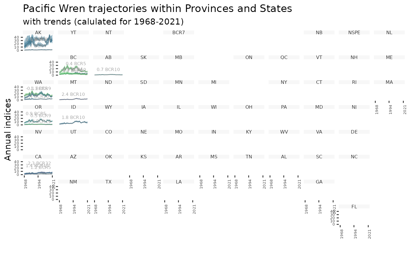
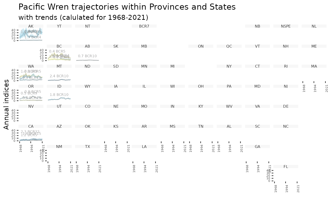 plot_geofacet(i, trends = t, multiple = TRUE, col_viridis = TRUE)
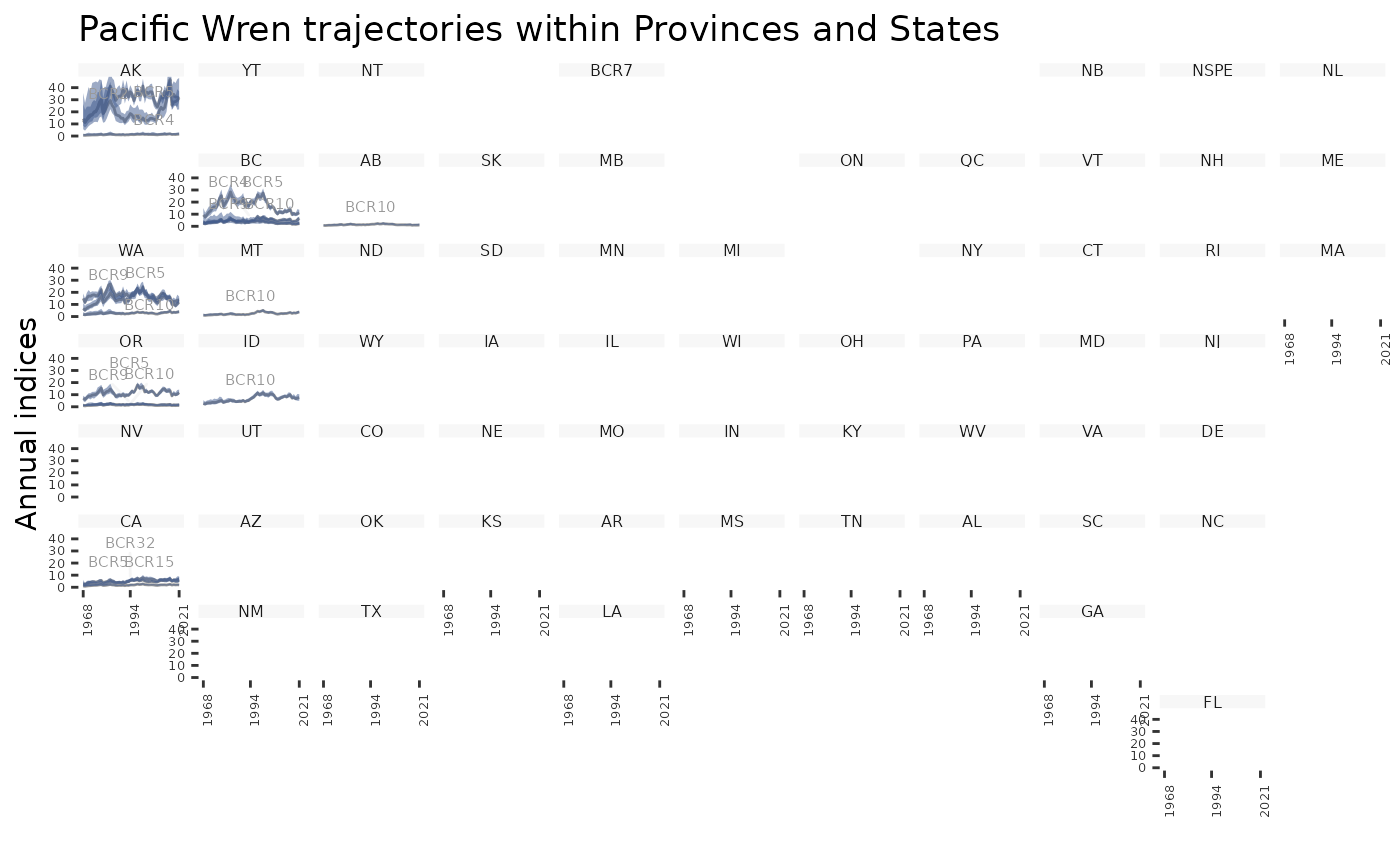
 plot_geofacet(i, multiple = TRUE)
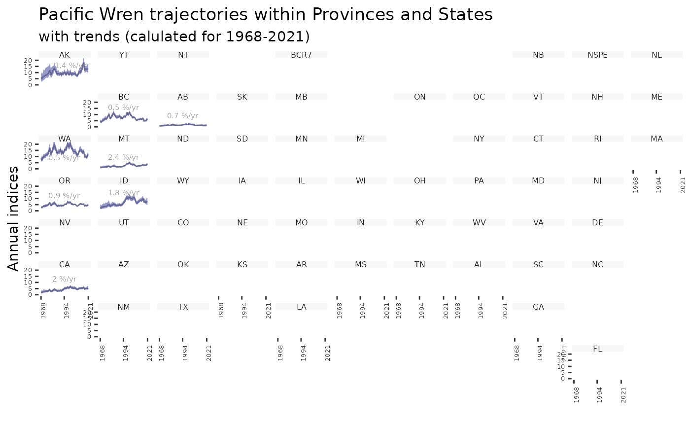
 plot_geofacet(i, trends = t, multiple = FALSE)
 plot_geofacet(i, multiple = FALSE)
 # With different ci_width, specify desired quantiles in indices
i <- generate_indices(pacific_wren_model,
regions = c("stratum", "prov_state"),
quantiles = c(0.005, 0.995))
#> Processing region stratum
#> Processing region prov_state
plot_geofacet(i, multiple = FALSE, ci_width = 0.99)
# With different ci_width, specify desired quantiles in indices
i <- generate_indices(pacific_wren_model,
regions = c("stratum", "prov_state"),
quantiles = c(0.005, 0.995))
#> Processing region stratum
#> Processing region prov_state
plot_geofacet(i, multiple = FALSE, ci_width = 0.99)
