Generates the indices plot for each stratum modelled.
Usage
plot_indices(
  indices = NULL,
  ci_width = 0.95,
  min_year = NULL,
  max_year = NULL,
  title = TRUE,
  title_size = 20,
  axis_title_size = 18,
  axis_text_size = 16,
  line_width = 1,
  add_observed_means = FALSE,
  add_number_routes = FALSE,
  indices_list,
  species
)
Arguments
- indices
List. Indices generated by
generate_indices().- ci_width
Numeric. Quantile defining the width of the plotted credible interval. Defaults to 0.95 (lower = 0.025 and upper = 0.975)
- min_year
Numeric. Minimum year to plot
- max_year
Numeric. Maximum year to plot
- title
Logical. Whether to include a title on the plot.
- title_size
Numeric. Font size of plot title. Defaults to 20
- axis_title_size
Numeric. Font size of axis titles. Defaults to 18
- axis_text_size
Numeric. Font size of axis text. Defaults to 16
- line_width
Numeric. Size of the trajectory line. Defaults to 1
- add_observed_means
Logical. Whether to include points indicating the observed mean counts. Default
FALSE. Note: scale of observed means and annual indices may not match due to imbalanced sampling among routes- add_number_routes
Logical. Whether to superimpose plot over a dotplot showing the number of BBS routes included in each year. This is useful as a visual check on the relative data-density through time because in most cases the number of observations increases over time
- indices_list
Deprecated. Use
indicesinstead- species
Defunct. Use
titleinstead
Examples
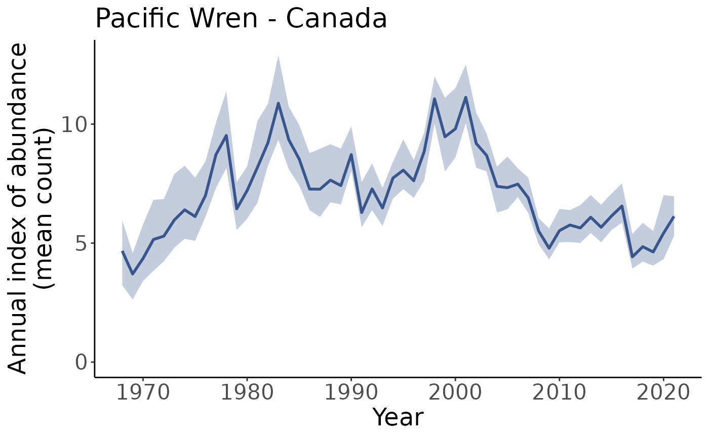
# Using the example model for Pacific Wrens...

# Generate country, continent, and stratum indices
i <- generate_indices(model_output = pacific_wren_model,
                      regions = c("country", "continent", "stratum"))
#> Processing region country
#> Processing region continent
#> Processing region stratum

# Now, plot_indices() will generate a list of plots for all regions
plots <- plot_indices(i)

# To view any plot, use [[i]]
plots[[1]]


names(plots)
#>  [1] "Canada"                   "United_States_of_America"
#>  [3] "continent"                "CA_AB_10"
#>  [5] "CA_BC_10"                 "CA_BC_4"
#>  [7] "CA_BC_5"                  "CA_BC_9"
#>  [9] "US_AK_2"                  "US_AK_4"
#> [11] "US_AK_5"                  "US_CA_15"
#> [13] "US_CA_32"                 "US_CA_5"
#> [15] "US_ID_10"                 "US_MT_10"
#> [17] "US_OR_10"                 "US_OR_5"
#> [19] "US_OR_9"                  "US_WA_10"
#> [21] "US_WA_5"                  "US_WA_9"

# Suppose we wanted to access the continental plot. We could do so with
cont_plot <- plots[["continental"]]

# You can specify to only plot a subset of years using min_year and max_year

# Plots indices from 2015 onward
p_2015_min <- plot_indices(i, min_year = 2015)

#Plot up indices up to the year 2017
p_2017_max <- plot_indices(i, max_year = 2017)

#Plot indices between 2011 and 2016
p_2011_2016 <- plot_indices(i, min_year = 2011, max_year = 2016)
names(plots)
#> [1] "Canada" "United_States_of_America"
#> [3] "continent" "CA_AB_10"
#> [5] "CA_BC_10" "CA_BC_4"
#> [7] "CA_BC_5" "CA_BC_9"
#> [9] "US_AK_2" "US_AK_4"
#> [11] "US_AK_5" "US_CA_15"
#> [13] "US_CA_32" "US_CA_5"
#> [15] "US_ID_10" "US_MT_10"
#> [17] "US_OR_10" "US_OR_5"
#> [19] "US_OR_9" "US_WA_10"
#> [21] "US_WA_5" "US_WA_9"
# Suppose we wanted to access the continental plot. We could do so with
cont_plot <- plots[["continental"]]
# You can specify to only plot a subset of years using min_year and max_year
# Plots indices from 2015 onward
p_2015_min <- plot_indices(i, min_year = 2015)
#Plot up indices up to the year 2017
p_2017_max <- plot_indices(i, max_year = 2017)
#Plot indices between 2011 and 2016
p_2011_2016 <- plot_indices(i, min_year = 2011, max_year = 2016)