1 - Prepare Geographic Boundaries

Published

October 4, 2023

Setup

library(tidyverse)
library(sf)
library(rnaturalearth)

Prepare maps

Choose a projection that preserves Area
According to All About Birds, shouldn’t be breeding outside of Canada or US

Therefore use only North America, and, further, only BCRs that overlap breeding range.

Choosing a projection

Because we will be creating equal-area grids with which to summarize the eBird checklist data, we want to make sure that the spatial data we work with is projected in order to preserve area.

Often I use the Statistics Canada Lambert projection (CRS 3347), but it preserves shape more than area.

There is also the BC Albers projection (CRS 3005) which is an equal area projection. I think this should work, even if some of the data is not in BC.

Base map

base_map <- ne_states(country = c("United States of America", "Canada"),
                      returnclass = "sf")

# Let's use a smaller range
crop_to <- st_bbox(c(xmin = -135, xmax = -92, ymin = 24.54, ymax = 60))
base_map <- st_crop(base_map, crop_to) |>
  st_make_valid() |>
  summarize() |>
  st_transform(3005)

Warning: attribute variables are assumed to be spatially constant throughout
all geometries

write_rds(base_map, "Data/Datasets/base_map.rds")

BCR maps

Acquired from Birds Canada NABCI Bird Conservation Regions
Should be cited

Bird Studies Canada and NABCI. 2014. Bird Conservation Regions. Published by Bird Studies Canada on behalf of the North American Bird Conservation Initiative. https://birdscanada.org/bird-science/nabci-bird-conservation-regions Accessed: 2023-10-04

Download and extract the data

download.file("https://birdscanada.org/download/gislab/bcr_terrestrial_shape.zip",
              destfile = "Data/bcr_maps.zip")
unzip("Data/bcr_maps.zip", exdir = "Data/")

Filter to relevant BCRs

bcr <- st_read("Data/BCR_Terrestrial/BCR_Terrestrial_master.shp") |>
  st_transform(3005) |>     # Stats Canada CRS
  rename_with(tolower) |>   # Lower case column names
  filter(bcr %in% c(9, 10, 11, 15, 16, 17, 18, 19)) |> # filter to relevant
  # Fix labels
  mutate(bcr = paste0(bcr,  " - ", str_to_title(bcrname)),
         bcr = factor(bcr, levels = unique(bcr)),
         province = str_to_title(province_s)) |>
  select(bcr, province, country)

Reading layer `BCR_Terrestrial_master' from data source 
  `/home/steffi/Projects/Business/Matt/lb_curlew_distribution/Data/BCR_Terrestrial/BCR_Terrestrial_master.shp' 
  using driver `ESRI Shapefile'
Simple feature collection with 373 features and 11 fields
Geometry type: MULTIPOLYGON
Dimension:     XY
Bounding box:  xmin: -179.1413 ymin: 14.53287 xmax: 179.7785 ymax: 83.11063
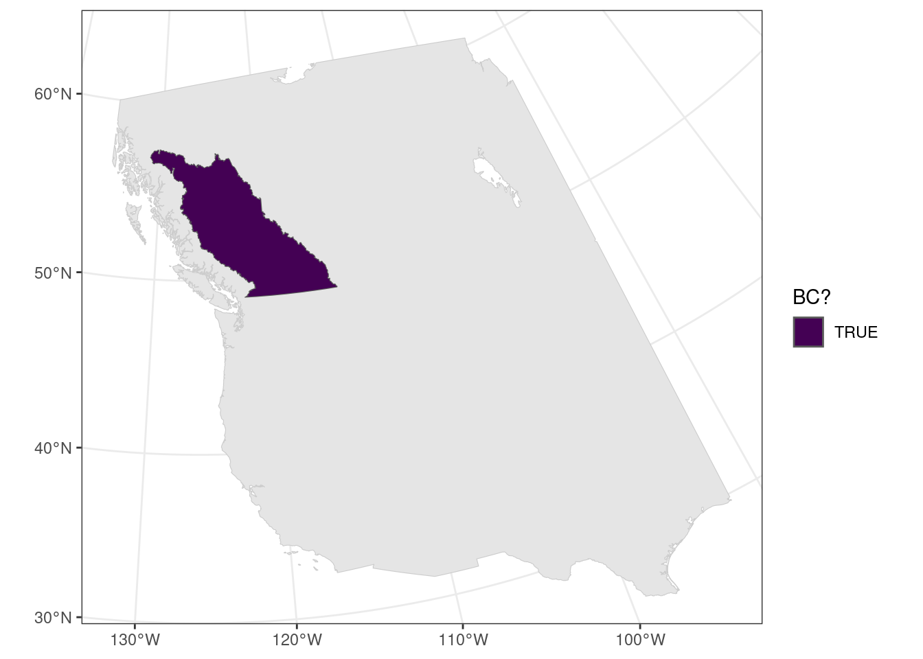
Geodetic CRS:  NAD83

# Get just BC within BCRs
bc <- filter(bcr, province == "British Columbia") |>
  summarize(bc = TRUE)

# Get just BCRs
bcr <- bcr |>
  select(-province, -country) |>
  group_by(bcr) |>
  summarize()

write_rds(bcr, "Data/Datasets/bcr_map.rds")
write_rds(bc, "Data/Datasets/bc_map.rds")

BCRs

ggplot() +
  theme_bw() +
  geom_sf(data = base_map, colour = "grey80") +
  geom_sf(data = bcr, aes(fill = bcr)) +
  scale_fill_viridis_d(name = "Bird Conservation Region")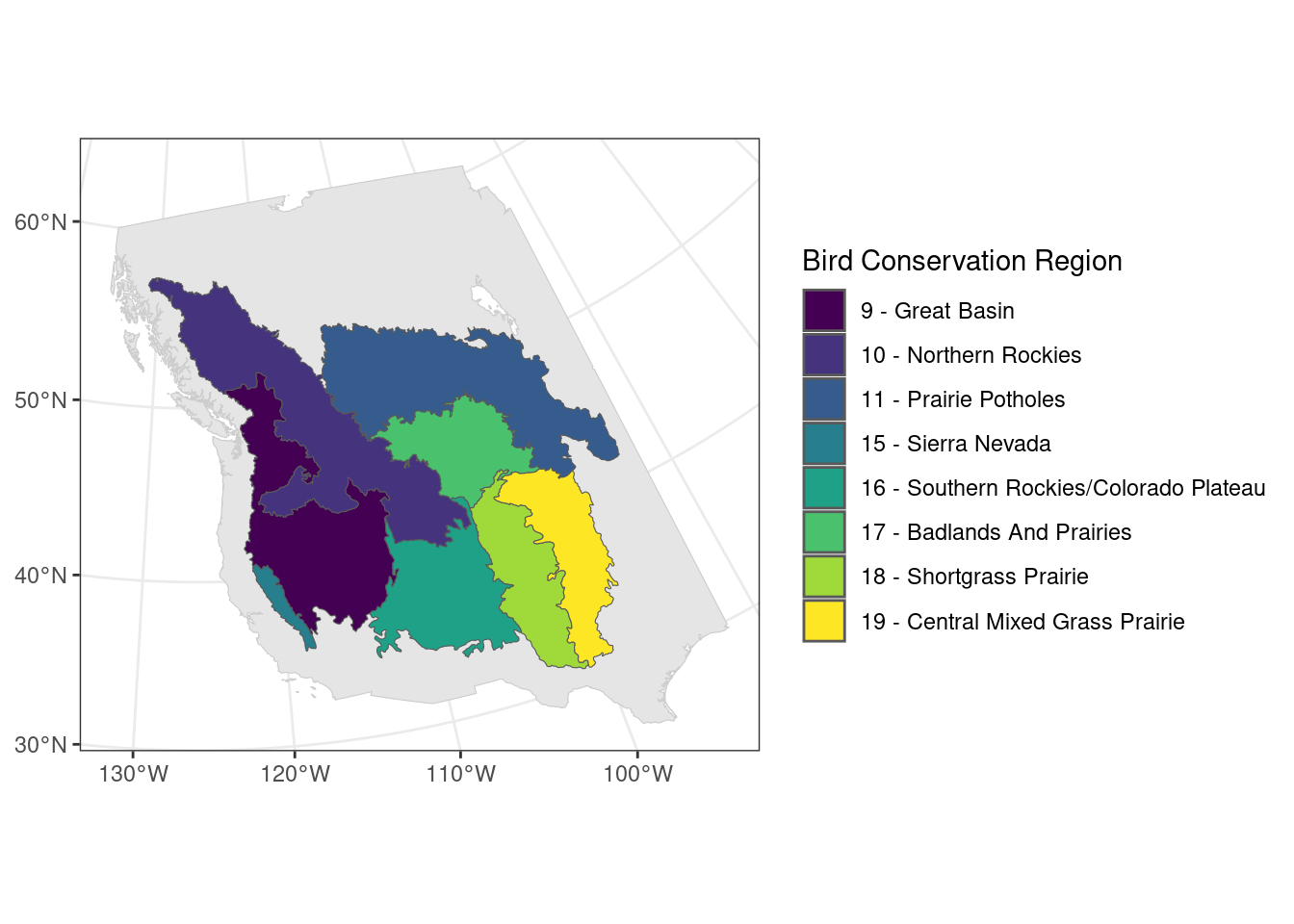

British Columbia

ggplot() +
  theme_bw() +
  geom_sf(data = base_map, colour = "grey80") +
  geom_sf(data = bc, aes(fill = bc)) +
  scale_fill_viridis_d(name = "BC?")