# A tibble: 344 × 8
   species island    bill_length_mm bill_depth_mm flipper_length_mm body_mass_g
   <fct>   <fct>              <dbl>         <dbl>             <int>       <int>
 1 Adelie  Torgersen           39.1          18.7               181        3750
 2 Adelie  Torgersen           39.5          17.4               186        3800
 3 Adelie  Torgersen           40.3          18                 195        3250
 4 Adelie  Torgersen           NA            NA                  NA          NA
 5 Adelie  Torgersen           36.7          19.3               193        3450
 6 Adelie  Torgersen           39.3          20.6               190        3650
 7 Adelie  Torgersen           38.9          17.8               181        3625
 8 Adelie  Torgersen           39.2          19.6               195        4675
 9 Adelie  Torgersen           34.1          18.1               193        3475
10 Adelie  Torgersen           42            20.2               190        4250
# ℹ 334 more rows
# ℹ 2 more variables: sex <fct>, year <int>Workshop: Dealing with Data in R
Visualizing Data in R
A primer on ggplot2
steffilazerte
@steffilazerte@fosstodon.org
@steffilazerte
steffilazerte.ca
![]()
Compiled: 2026-02-19
Outline
1. Figures with ggplot2 (A tidyverse package)
- Basic plot
- Common plot types
- Plotting by categories
- Adding statistics
- Customizing plots
- Annotating plots
2. Combining figures with patchwork
3. Saving figures

Our data set: Palmer Penguins!
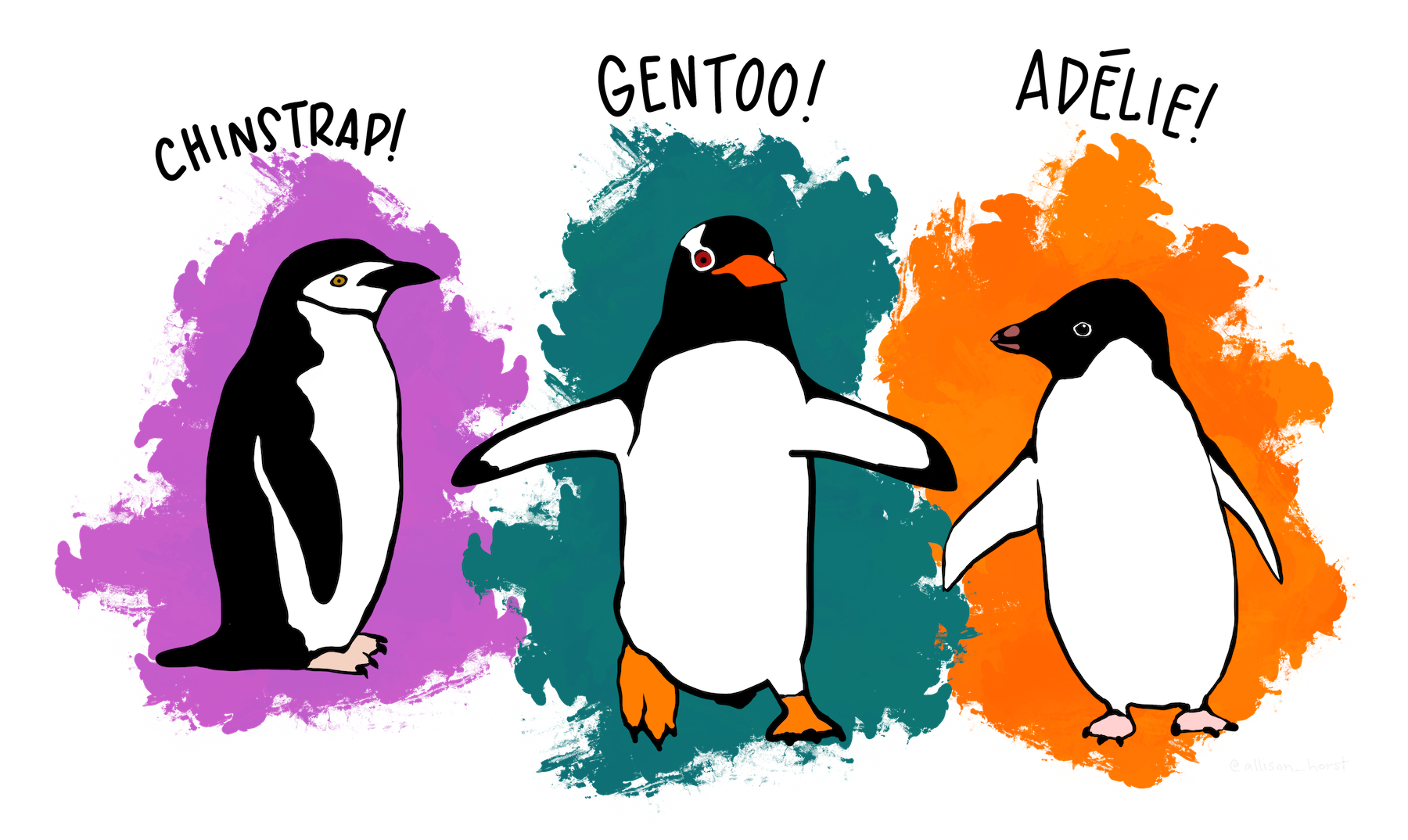

Artwork by @allison_horst
Our data set: Palmer Penguins!
Artwork by @allison_horst
Your turn!
Run this code and look at the output in the console
A basic plot
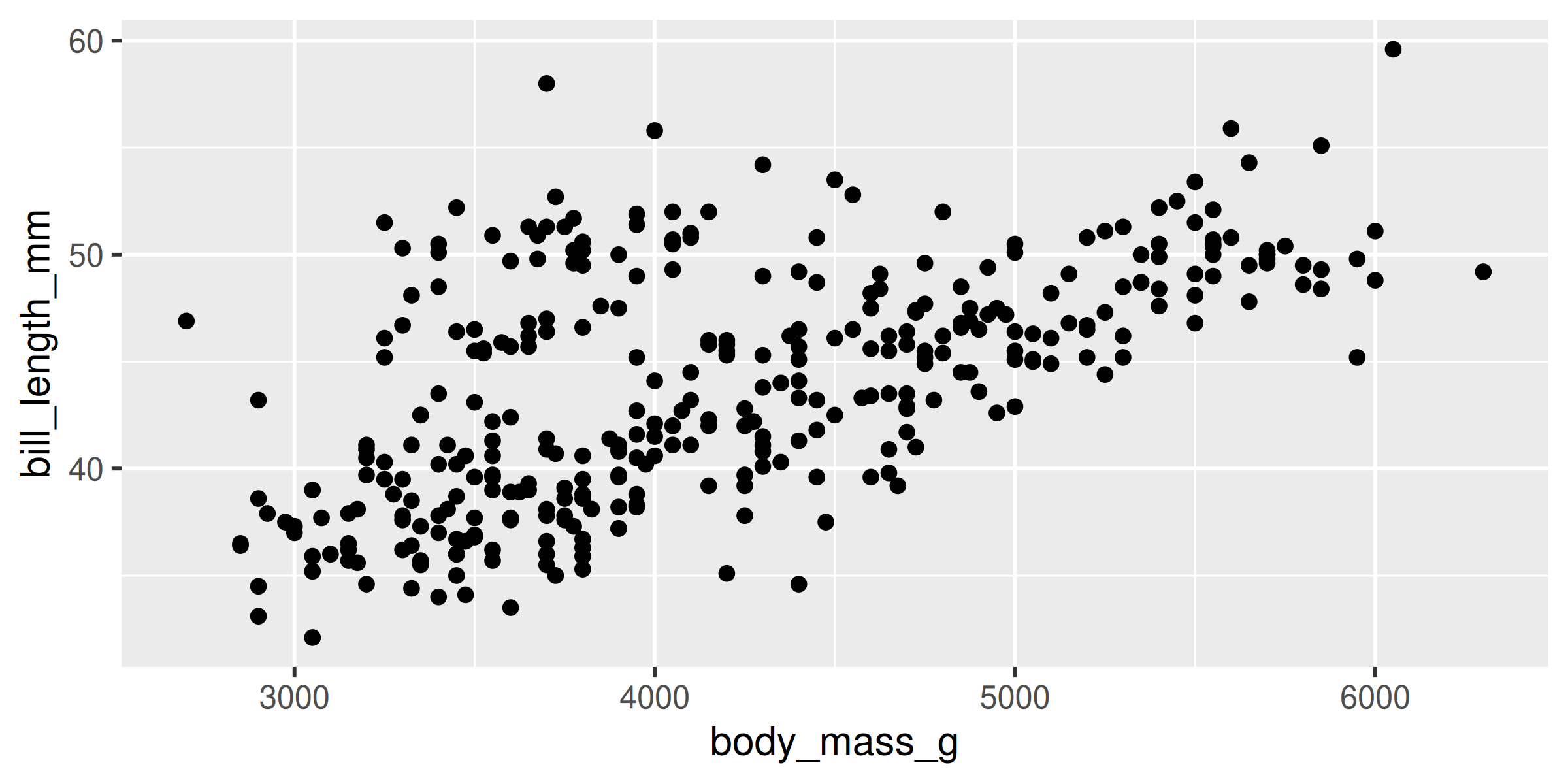
Break it down
library()
- Load the
palmerguinspackage - Now we have access to
penguinsdata
Break it down
library()
- Load the
tidyversepackages
(includesggplot2) - Now we have access to the
ggplot()function (andaes()andgeom_point()etc.)

Break it down
ggplot()
- Set the attributes of your plot
data= Datasetaes= Aesthetics (how the data are used)- Think of this as your plot defaults

Break it down
geom_point()
- Choose a
geomfunction to display the data - Always added to a
ggplot()call with+
ggplots are essentially layered objects, starting with a call to
ggplot()

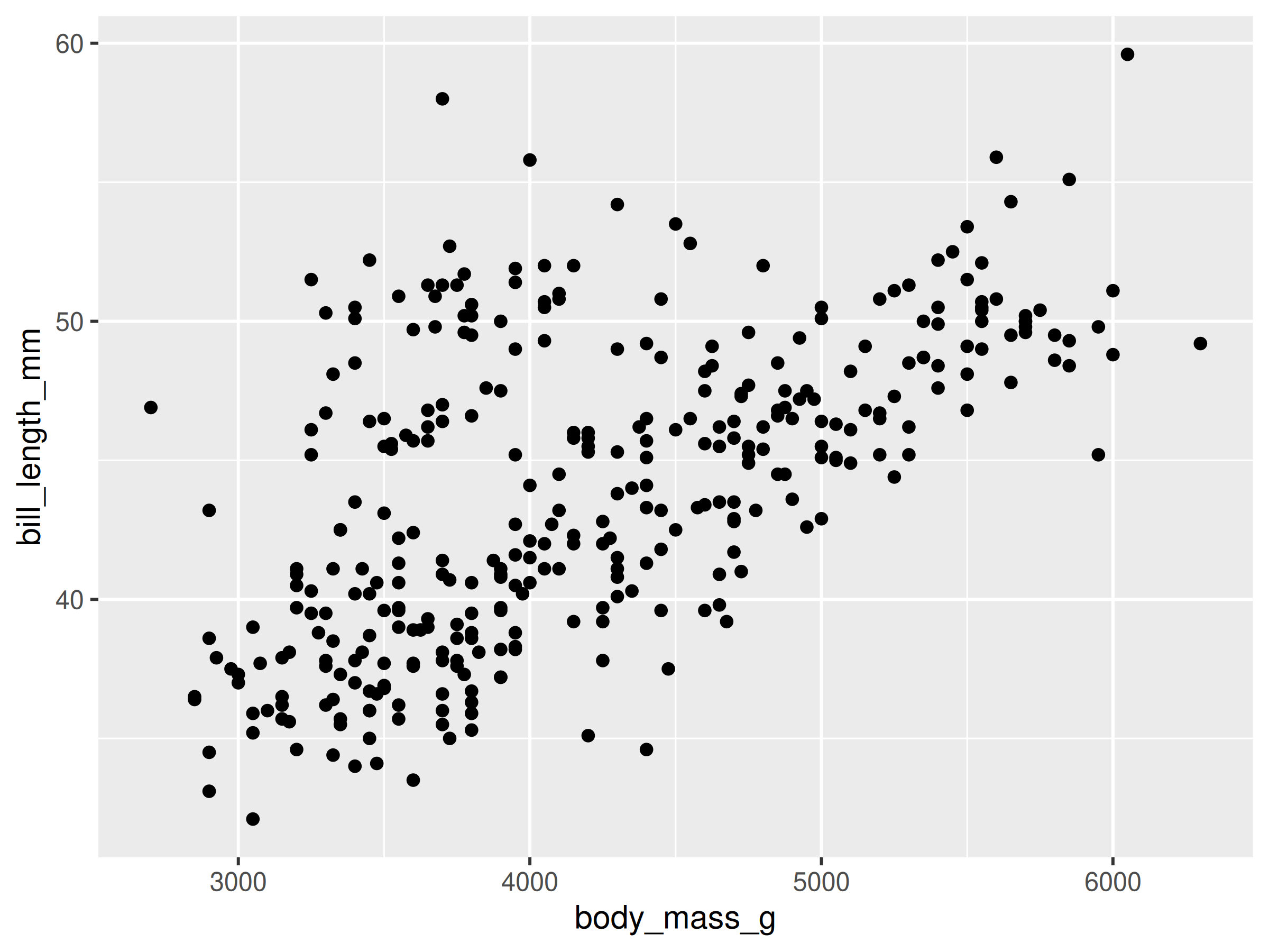
Plots are layered

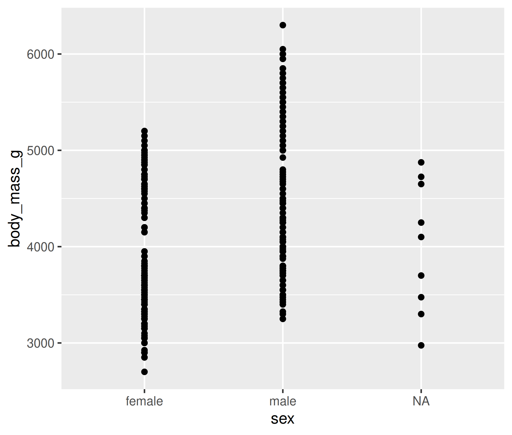
Plots are layered
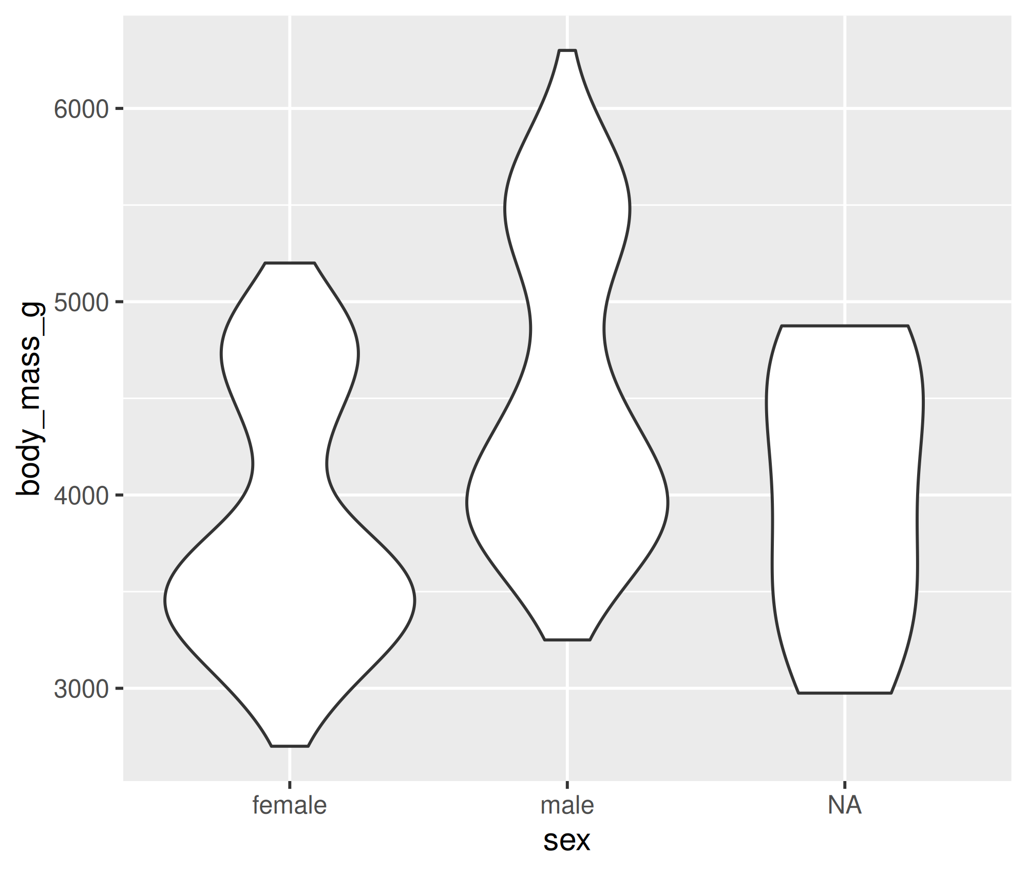
You can add multiple layers

Plots are objects
Any ggplot can be saved as an object
Geoms: Lines
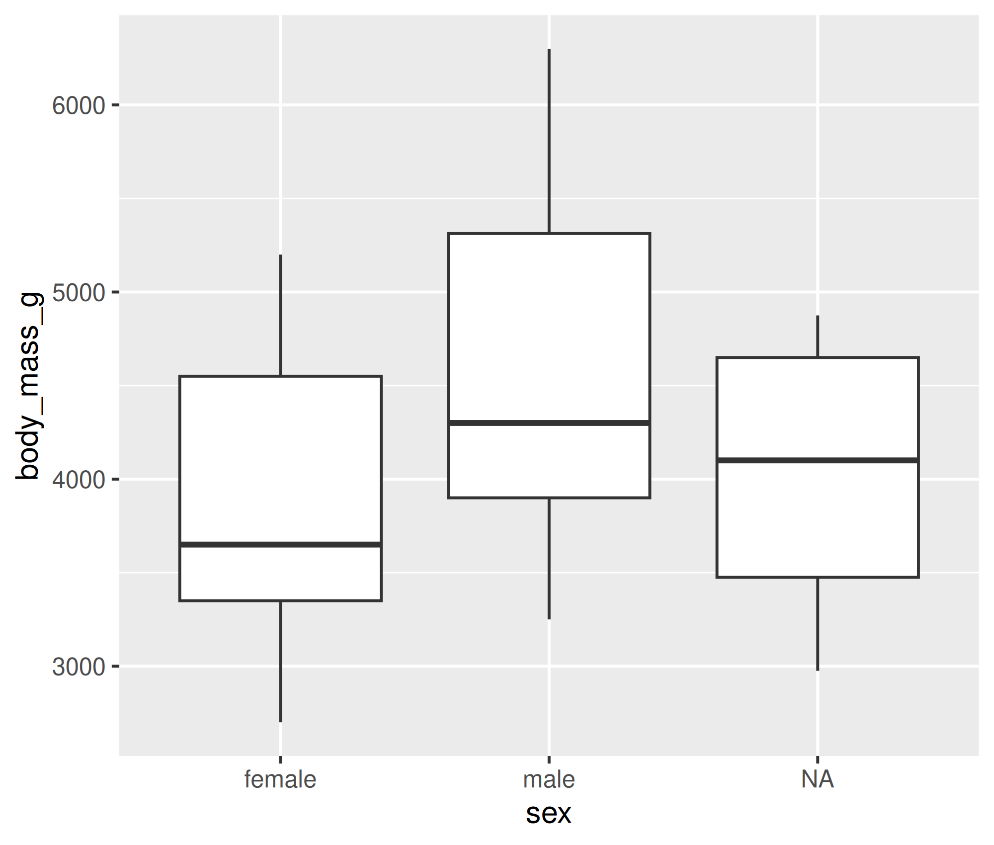
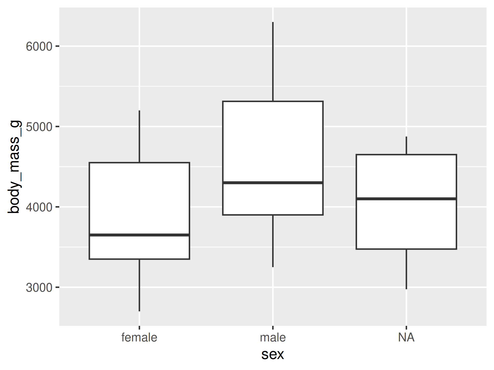
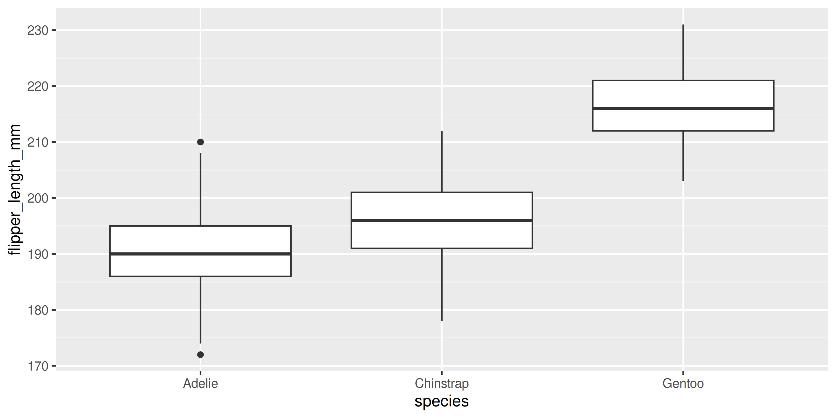
Geoms: Boxplots
Geoms: Histogram
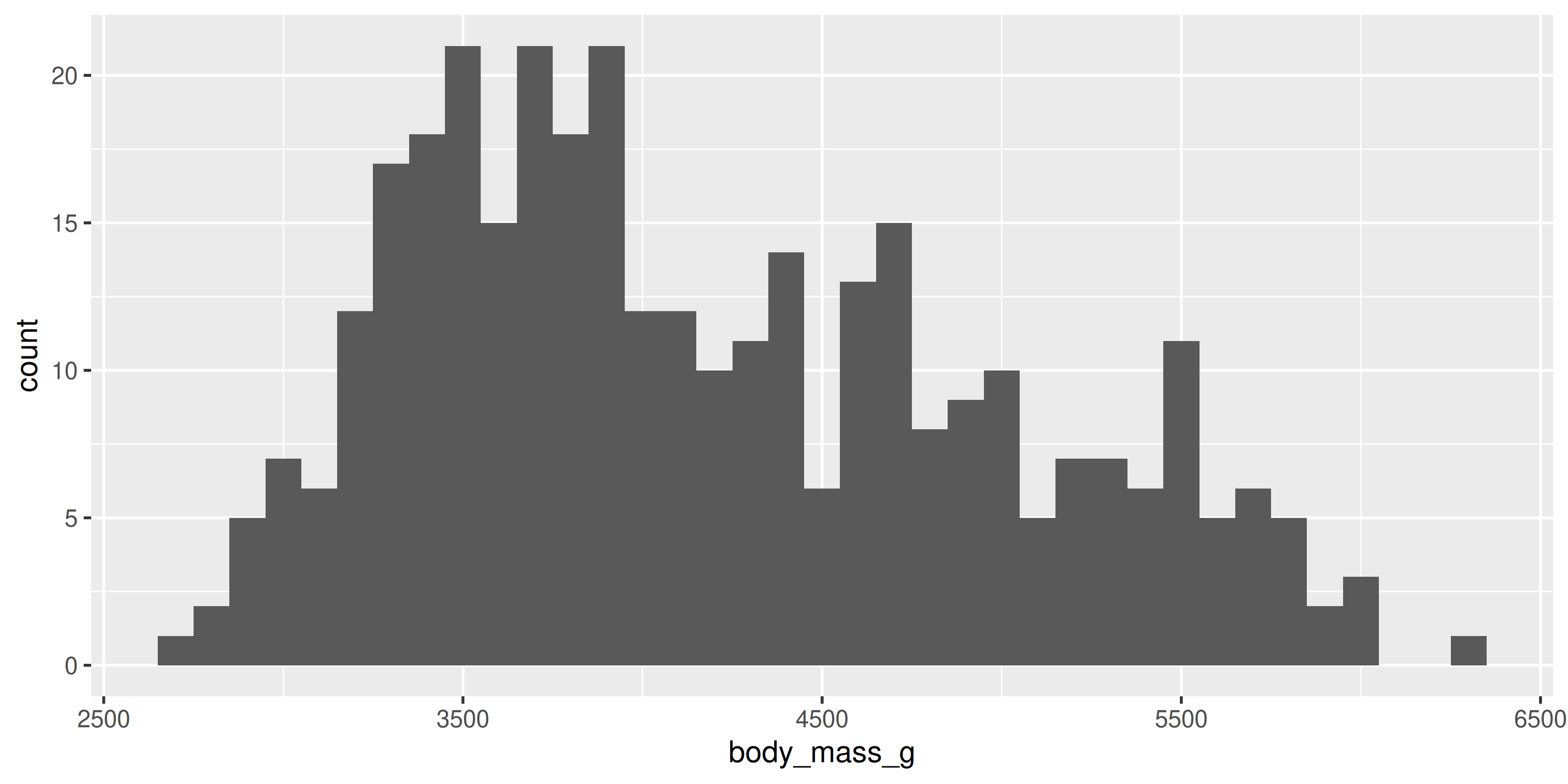
Note:
We only need 1 aesthetic here
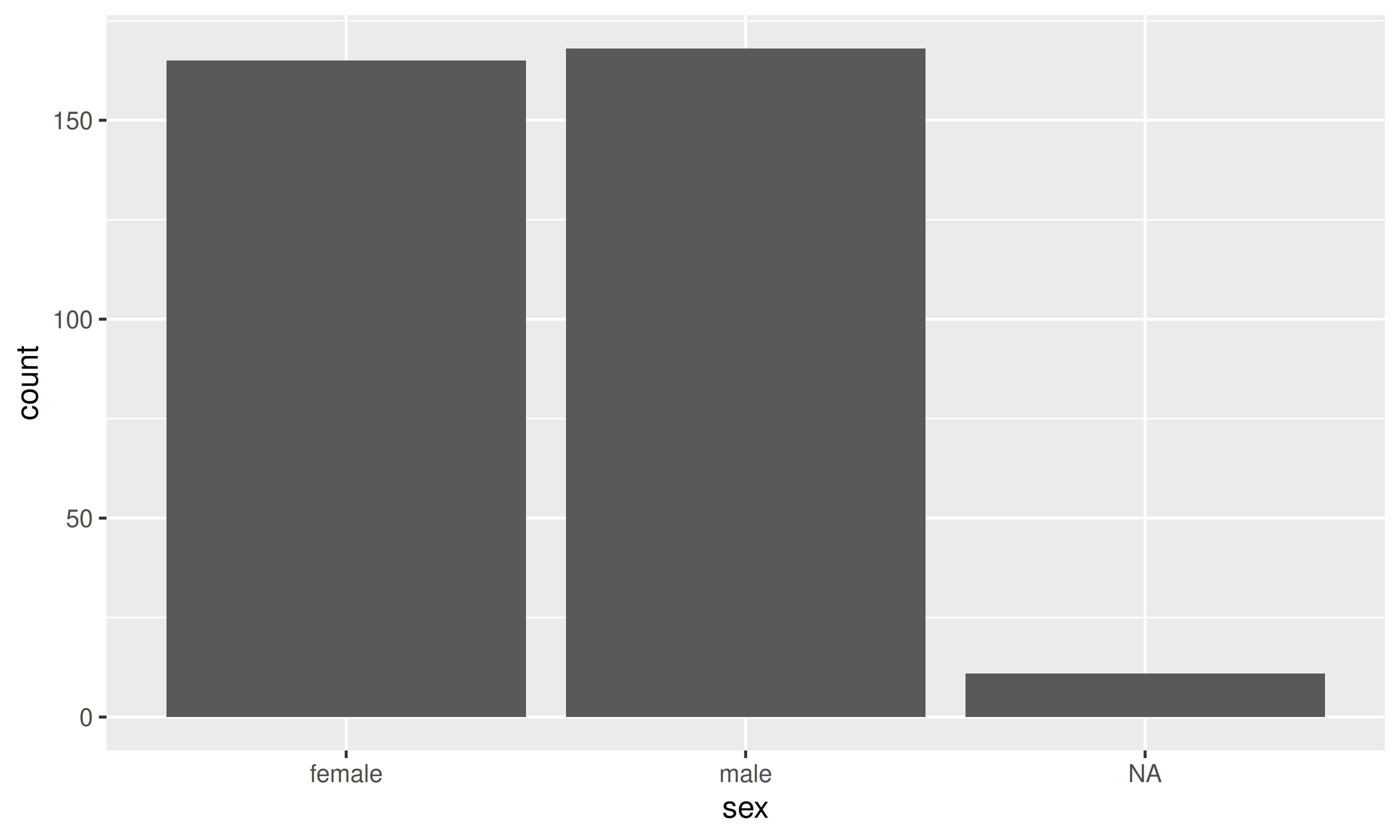
Geoms: Barplots
Let ggplot count your data
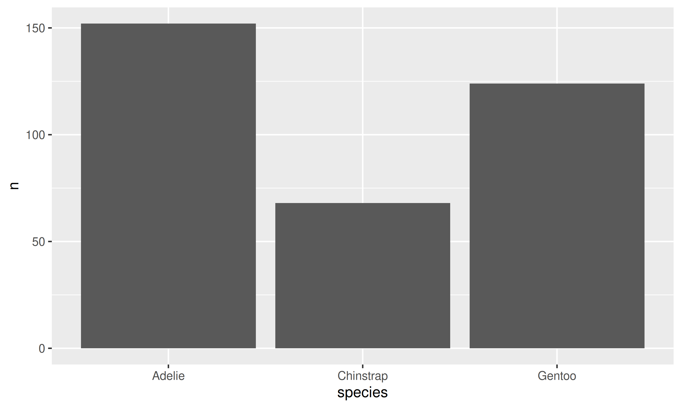
Geoms: Barplots
You can also provide the counts
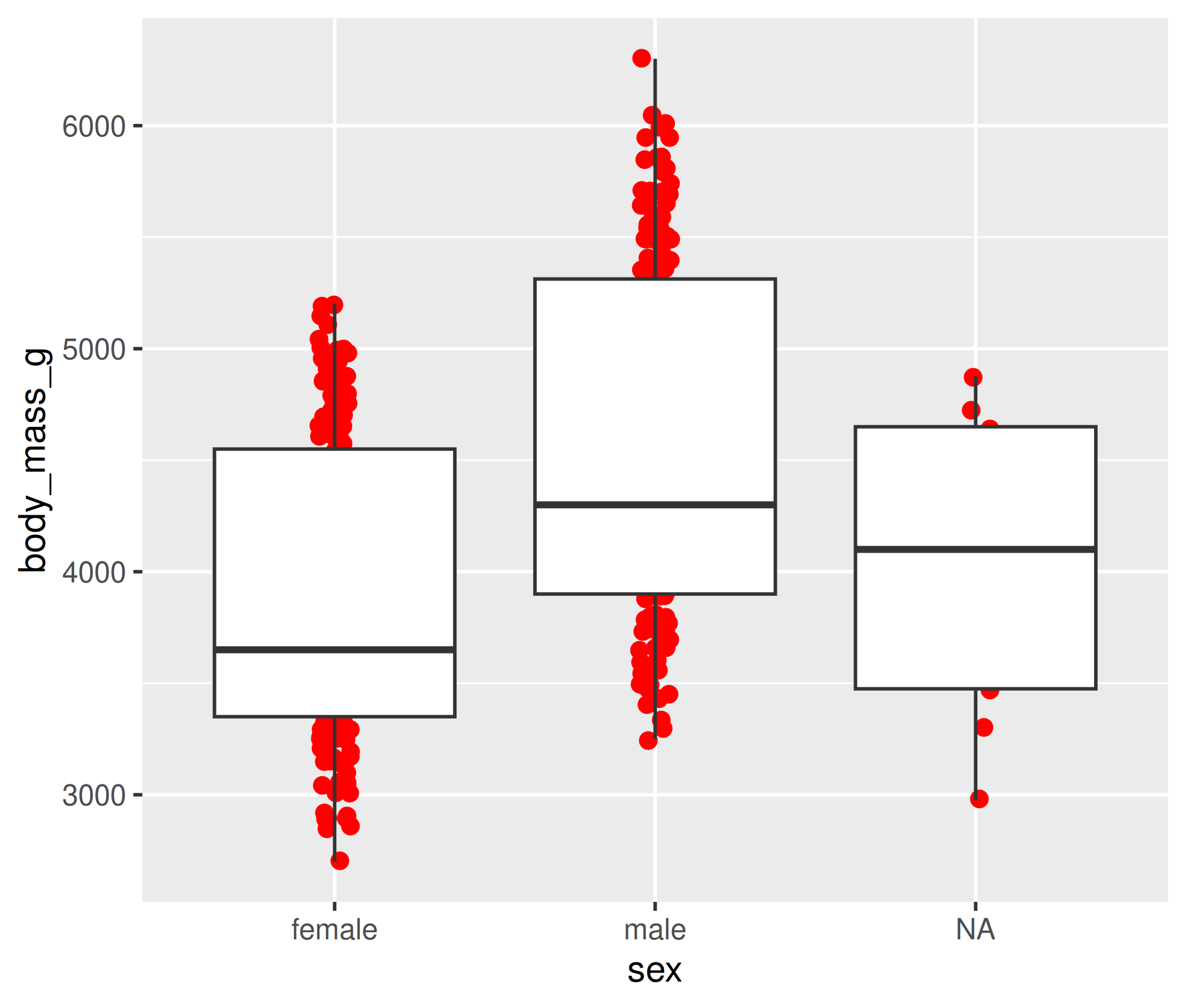
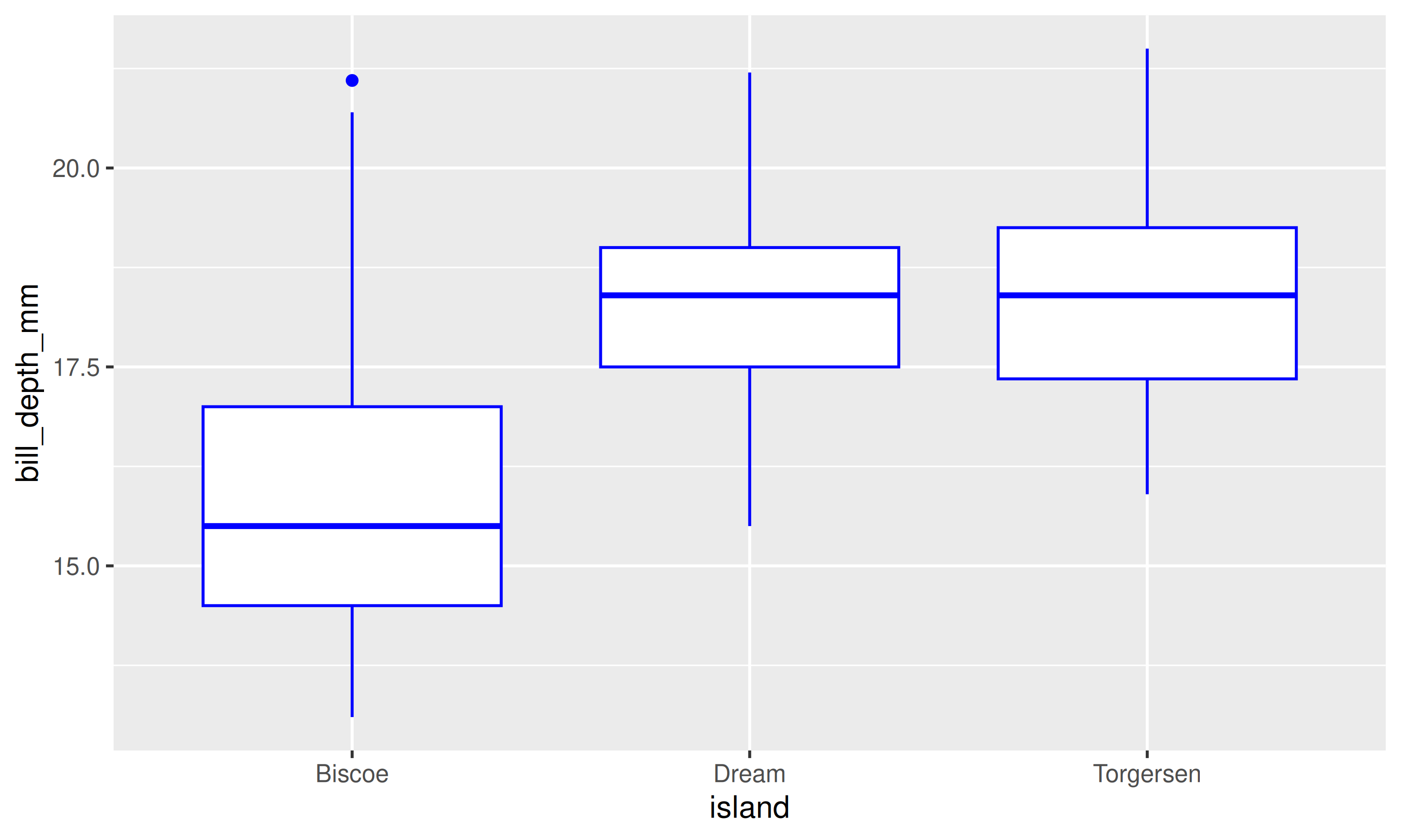
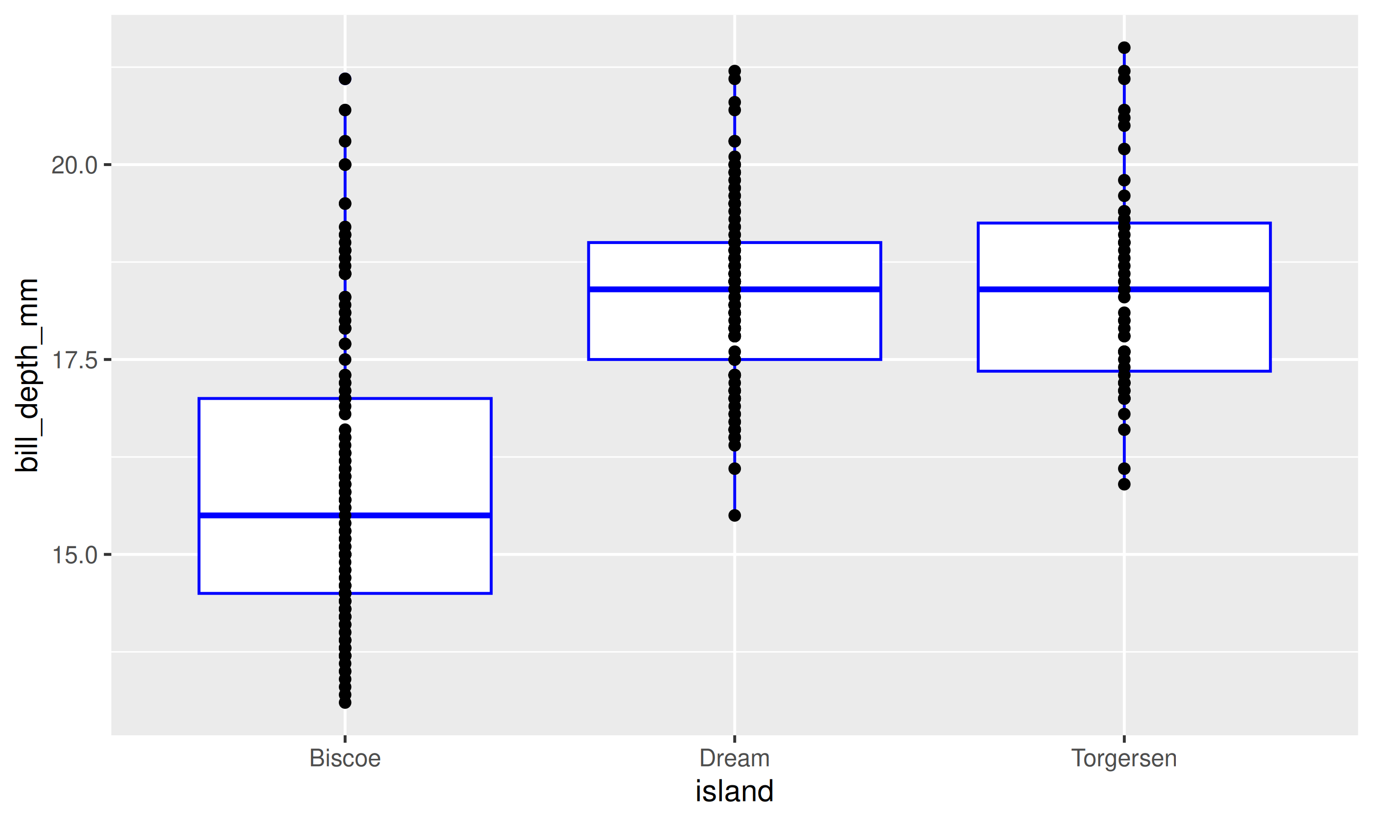
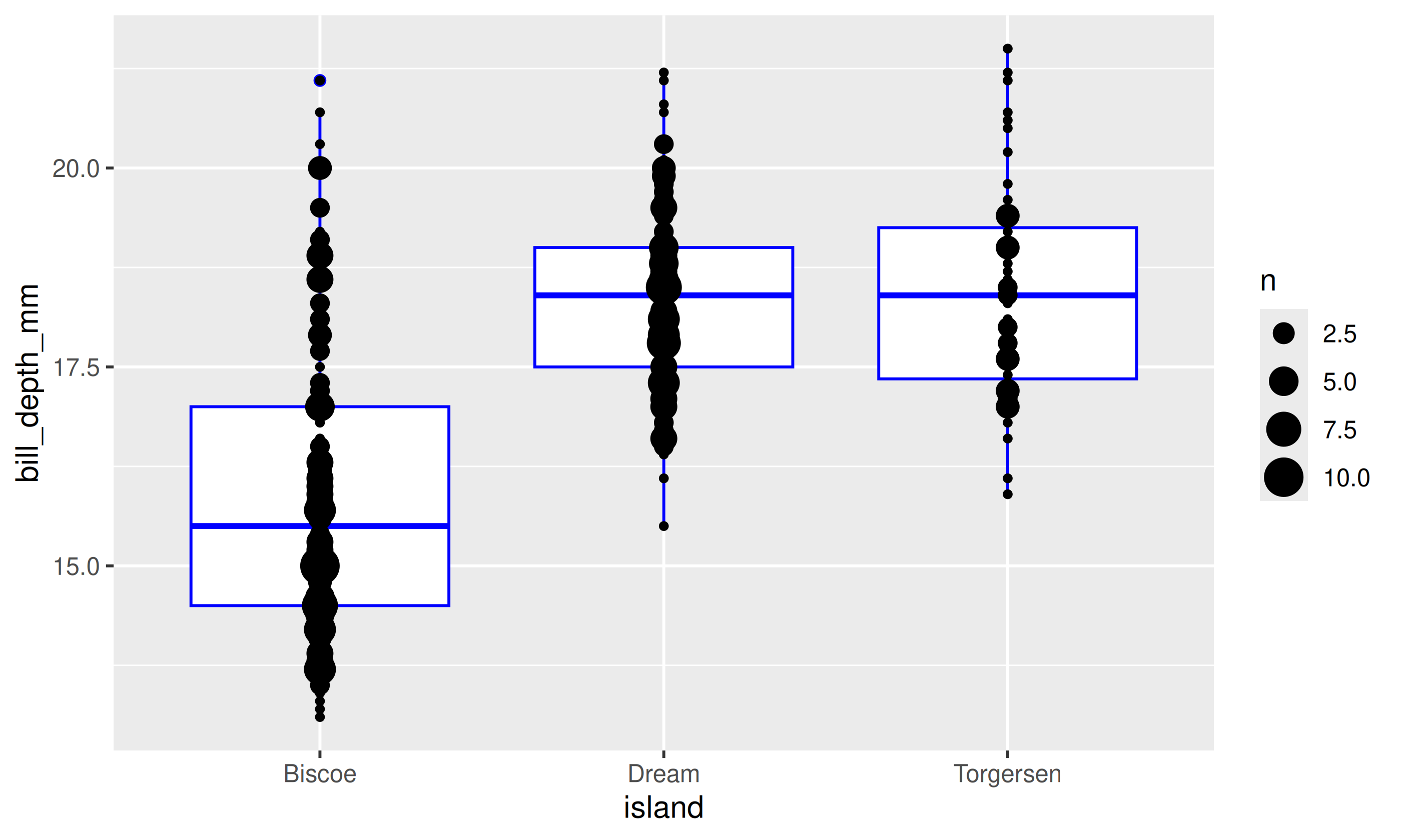
Your Turn: Create this plot
Too Easy?
Plot points on top
Why not consider jittering them?
Your Turn: Create this plot

Your Turn: Create this plot
Too Easy?
Your Turn: Create this plot
Too Easy?

Your Turn: Create this plot
Too Easy?
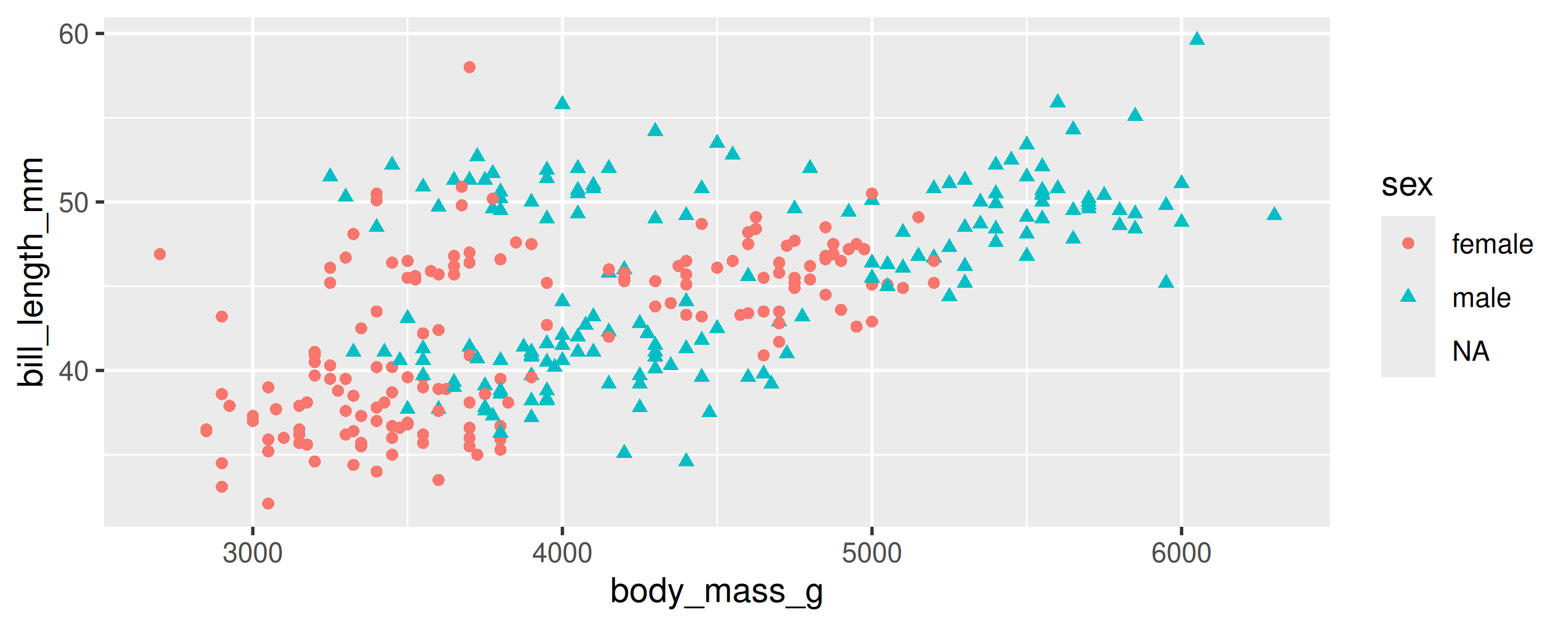
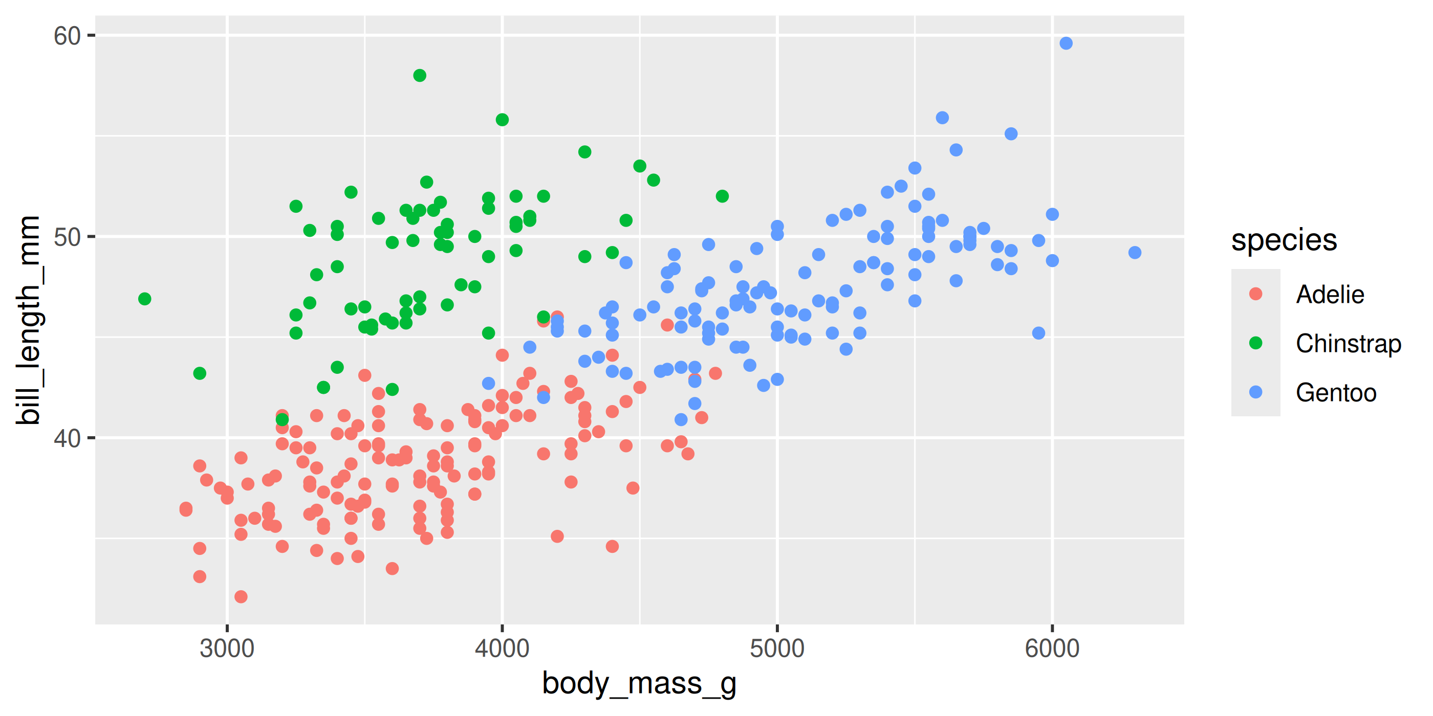
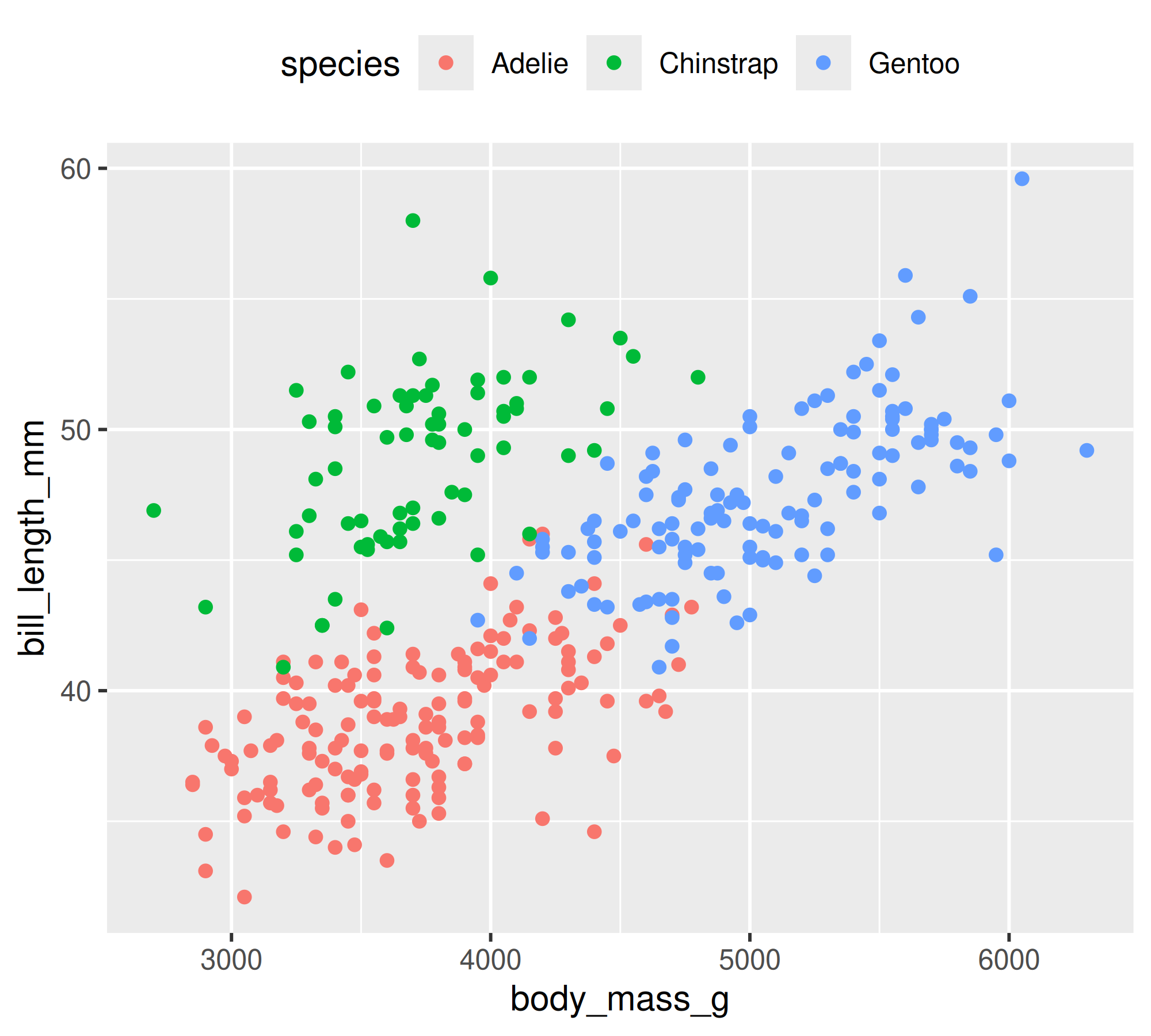
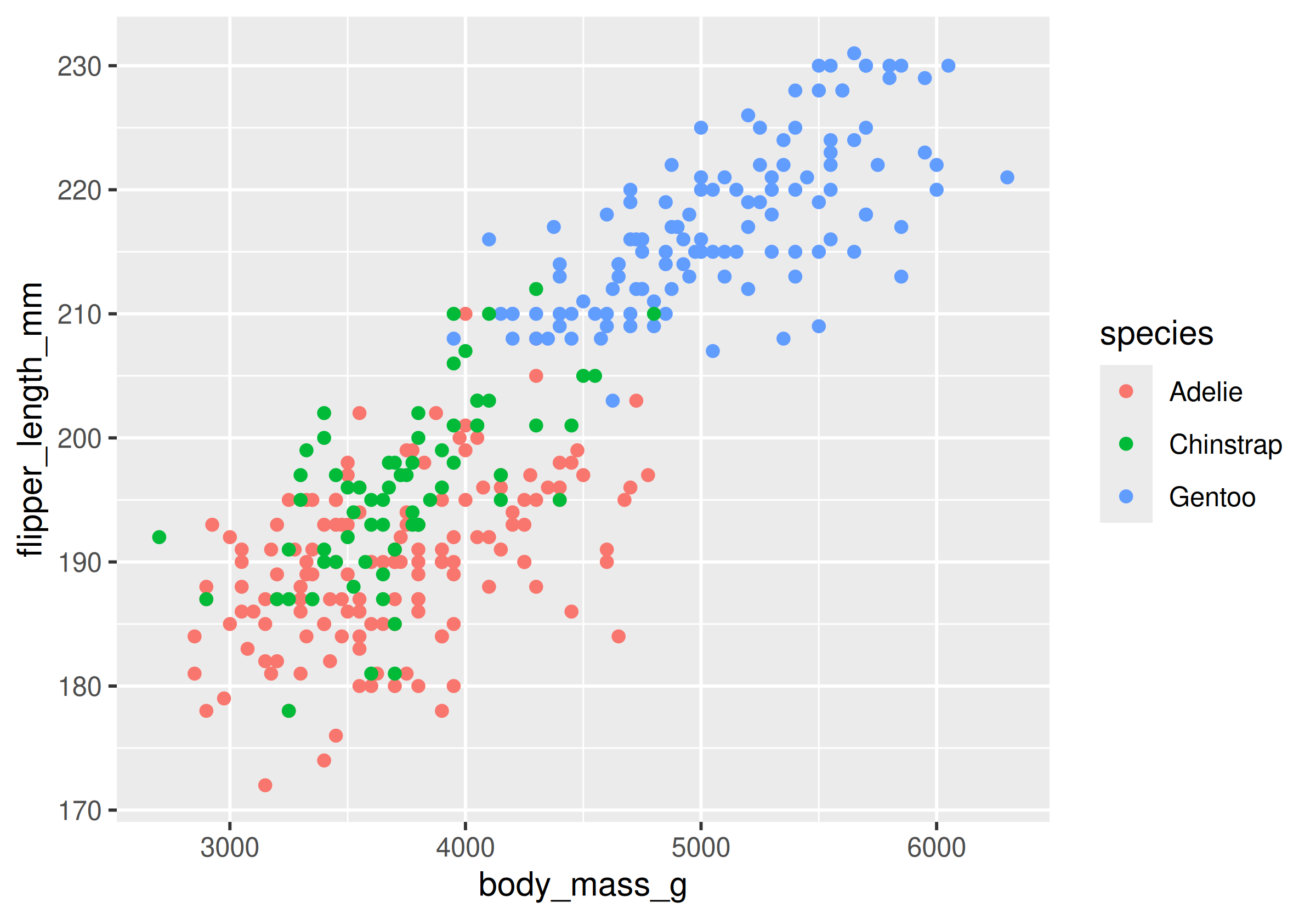
Mapping aesthetics
Mapping aesthetics
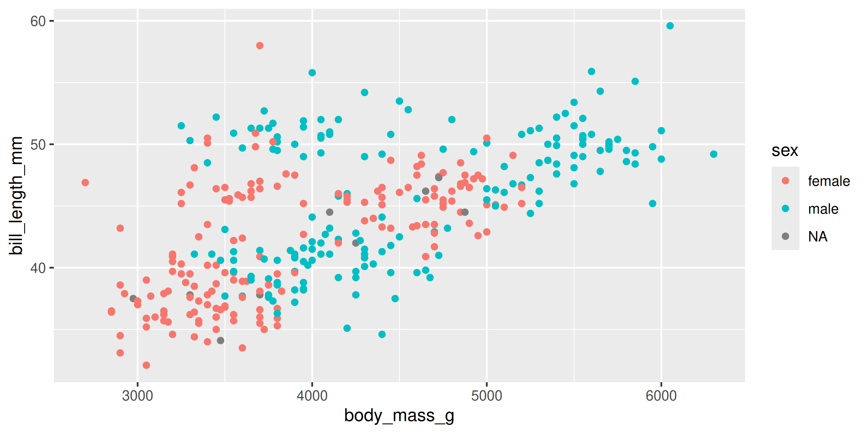
Mapping aesthetics
ggplot automatically populates the legends (combining where it can)
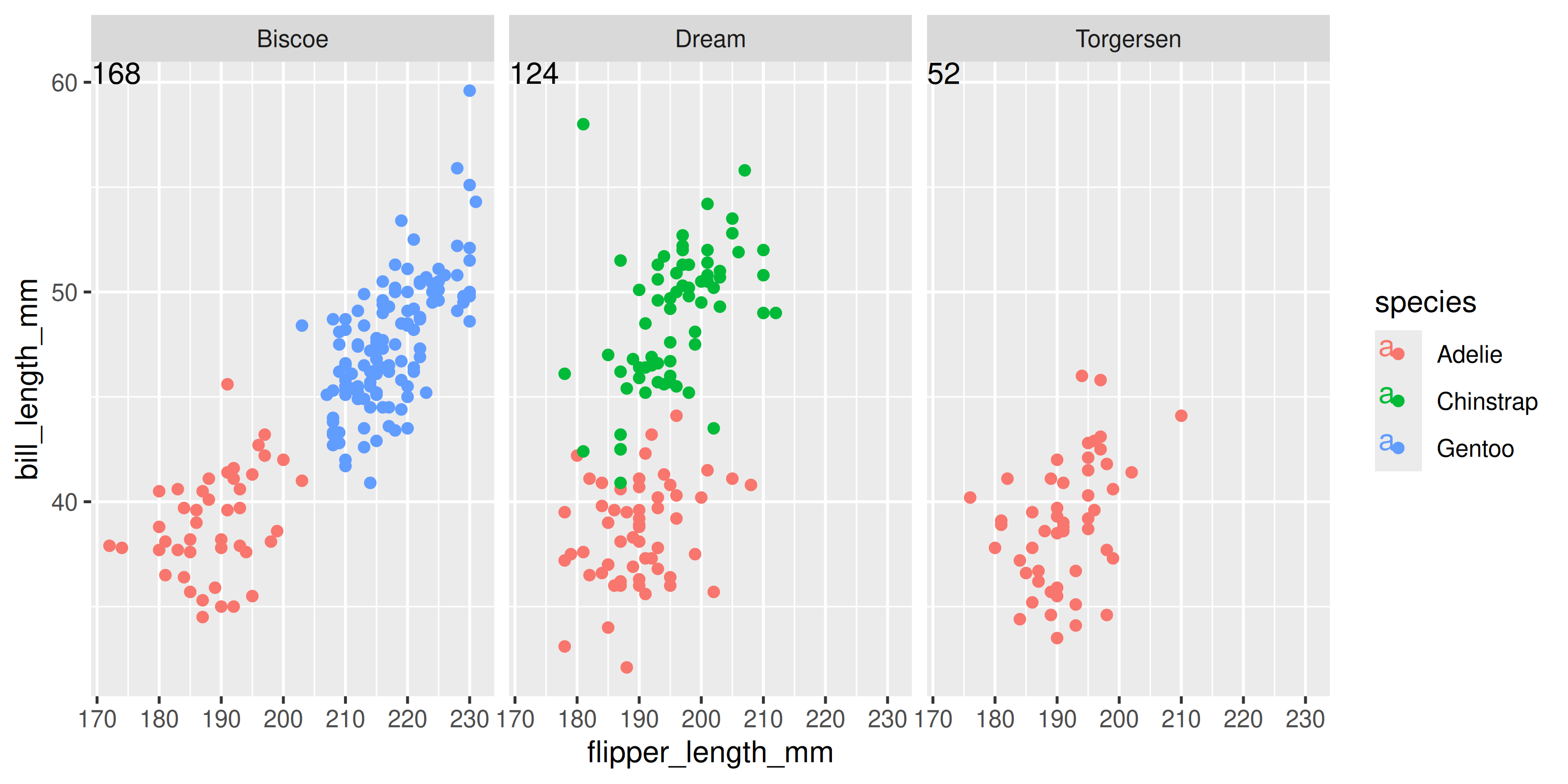
Faceting: facet_wrap()
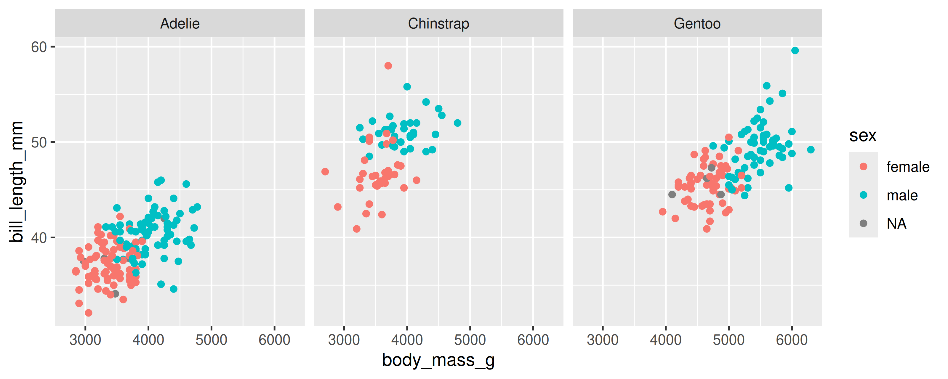
Split plots by one grouping variable
Faceting: facet_grid()
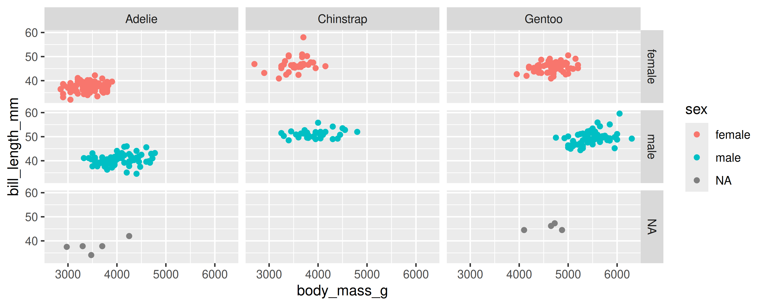
Split plots by two grouping variables
Your Turn: Create this plot

Hint:
colouris for outlining with a colour,fillis for ‘filling’ with a colour
Too Easy? Split boxplots by sex and island
Your Turn: Create this plot
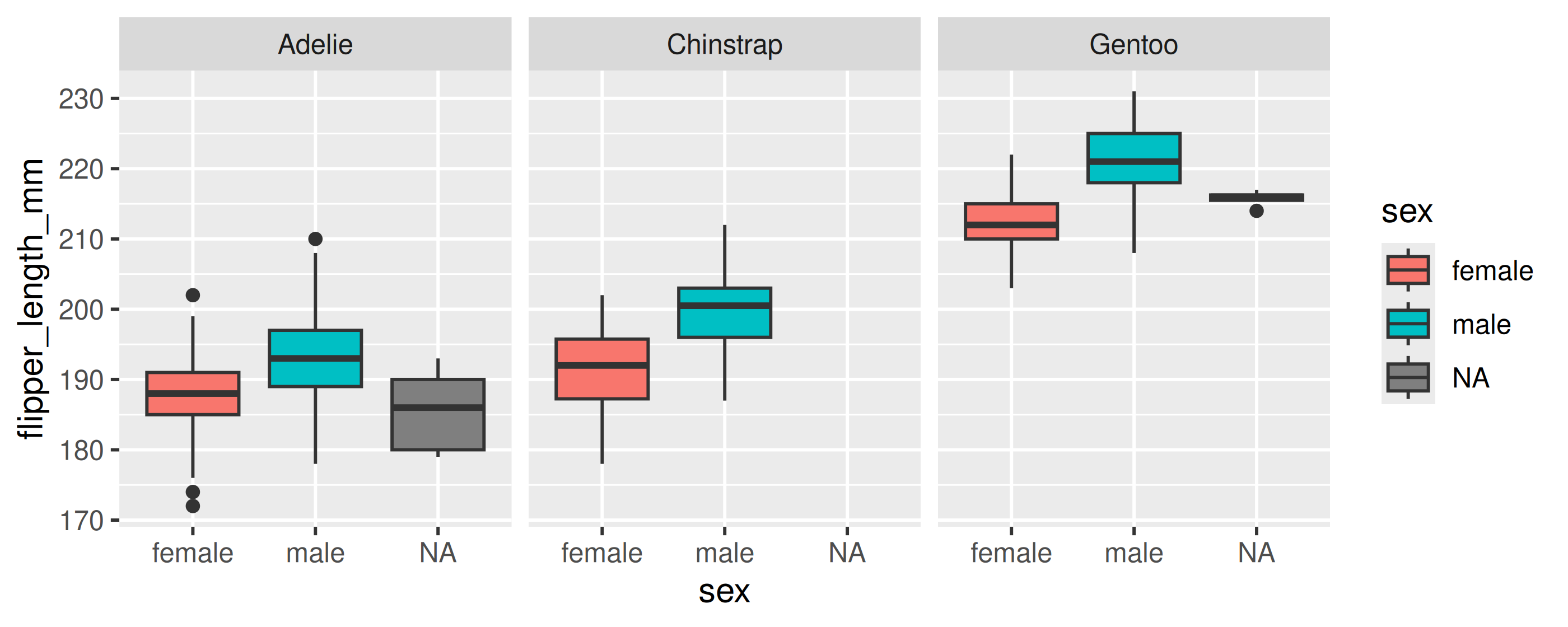
Hint:
colouris for outlining with a colour,fillis for ‘filling’ with a colour
Too Easy? Split boxplots by sex and island
Your Turn: Create this plot
Too Easy?
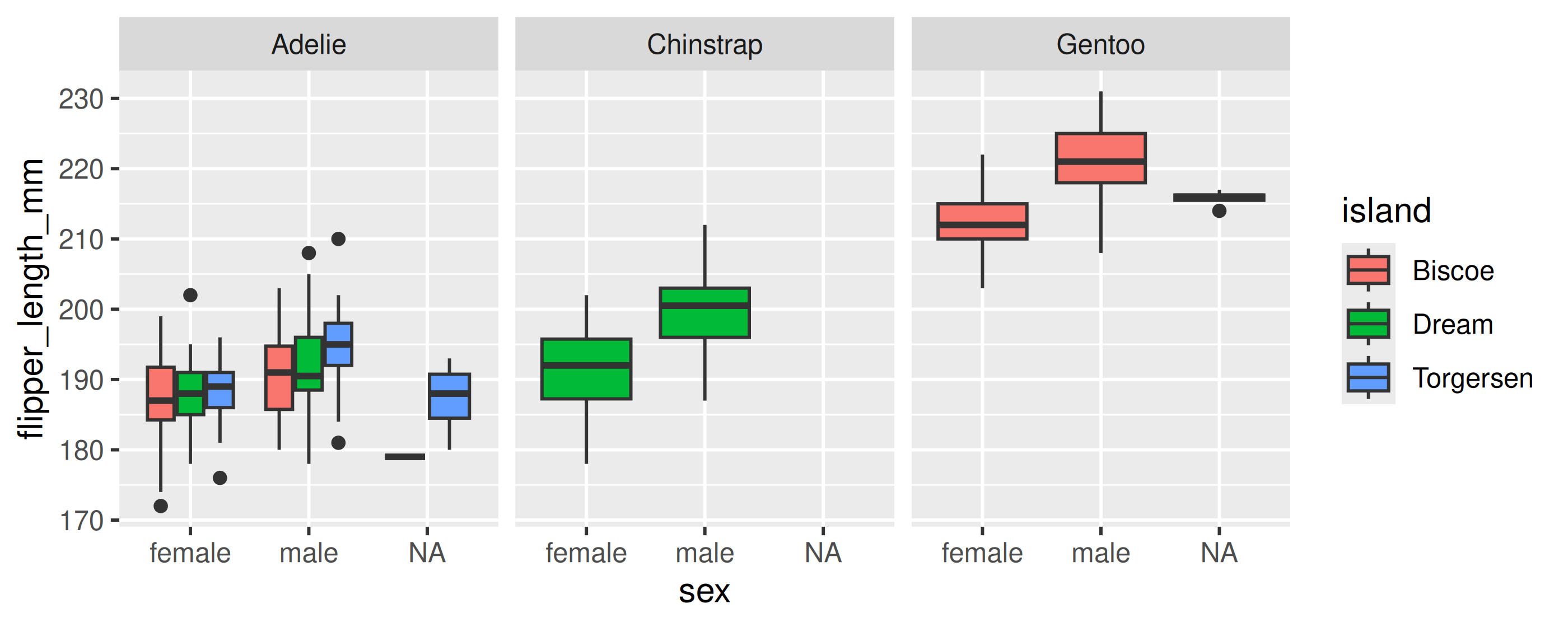
Small change (
fill = sextofill = island) results in completely different plot
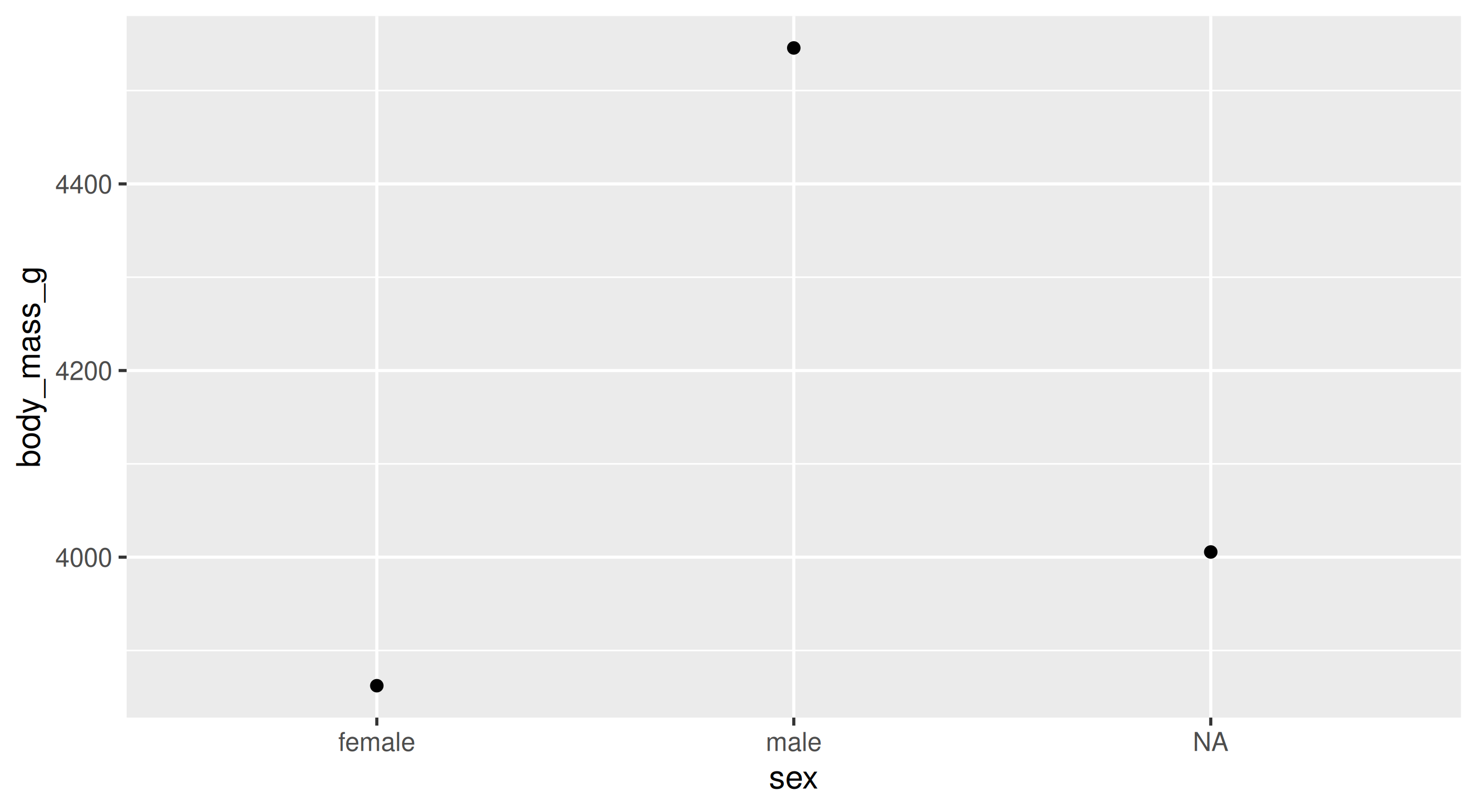
Summarizing data
Add data means as points
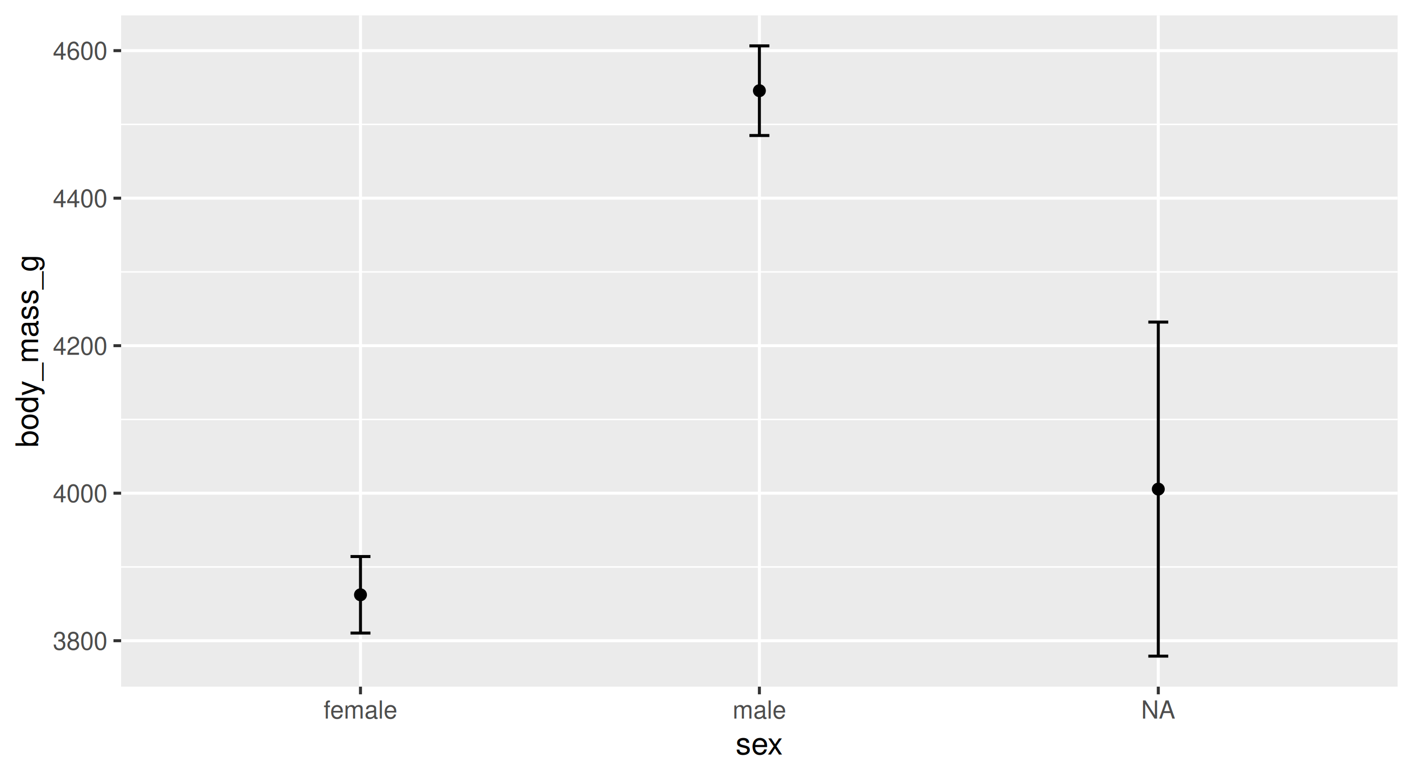
Summarizing data
Add error bars, calculated from the data
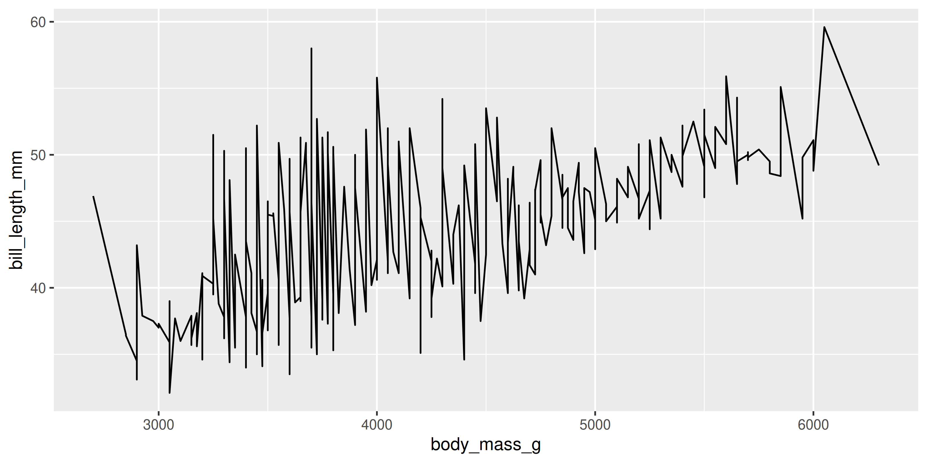
Trendlines / Regression lines
geom_line() is connect-the-dots, not a trend or linear model
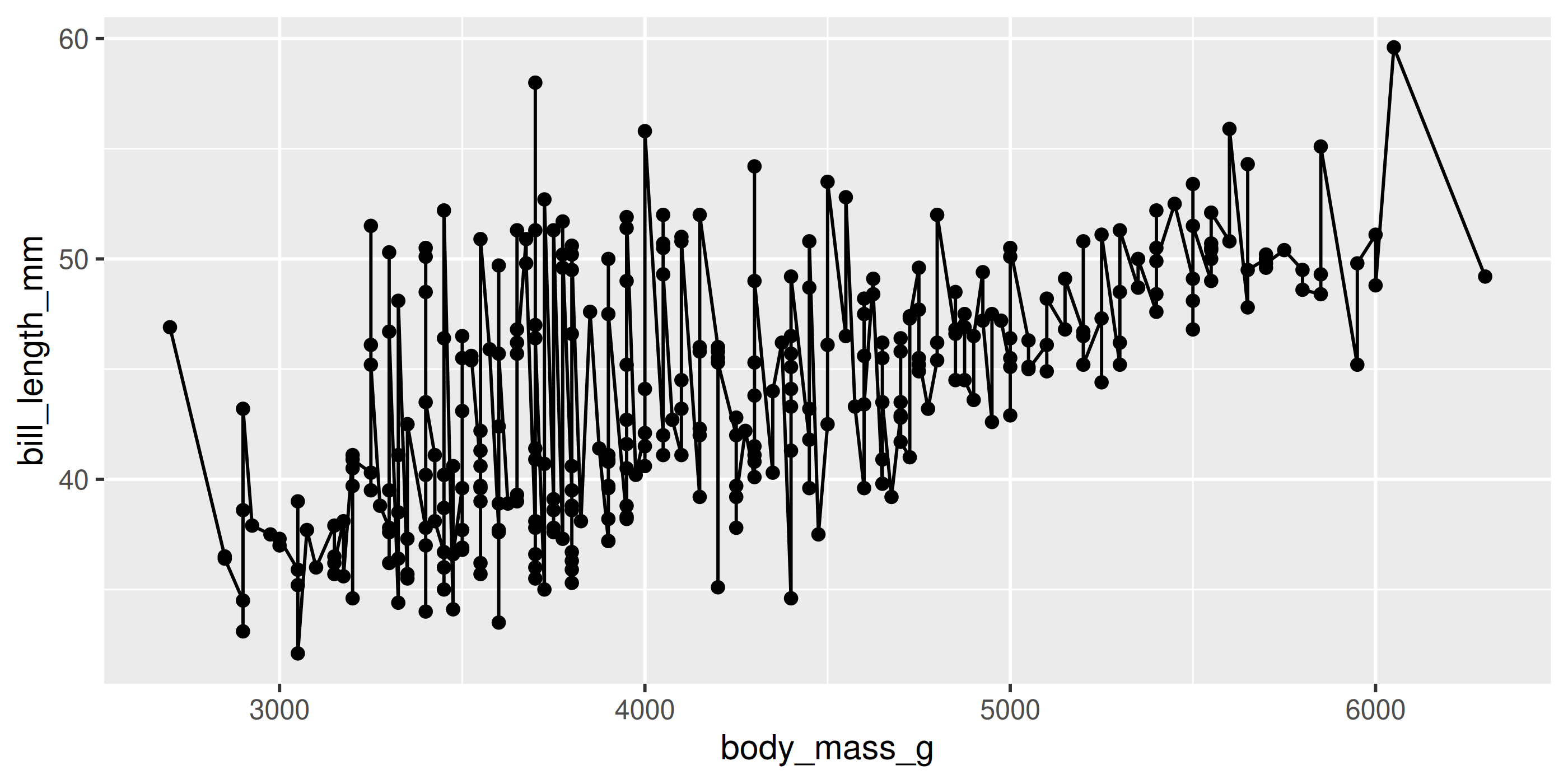
Not what we’re looking for
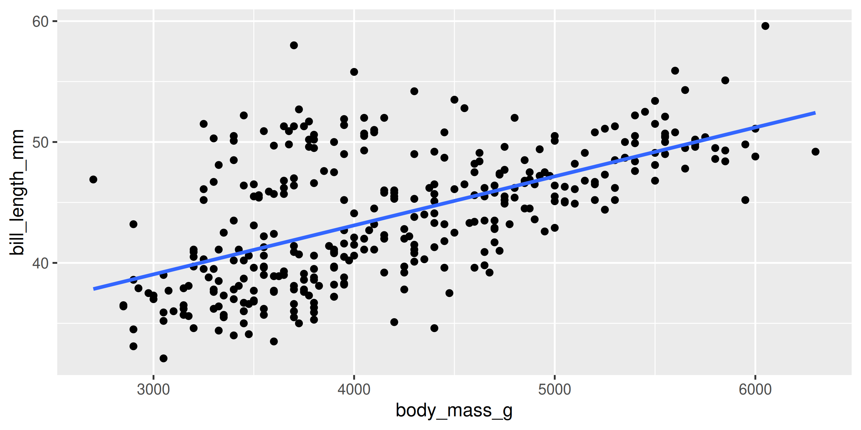
Trendlines / Regression lines
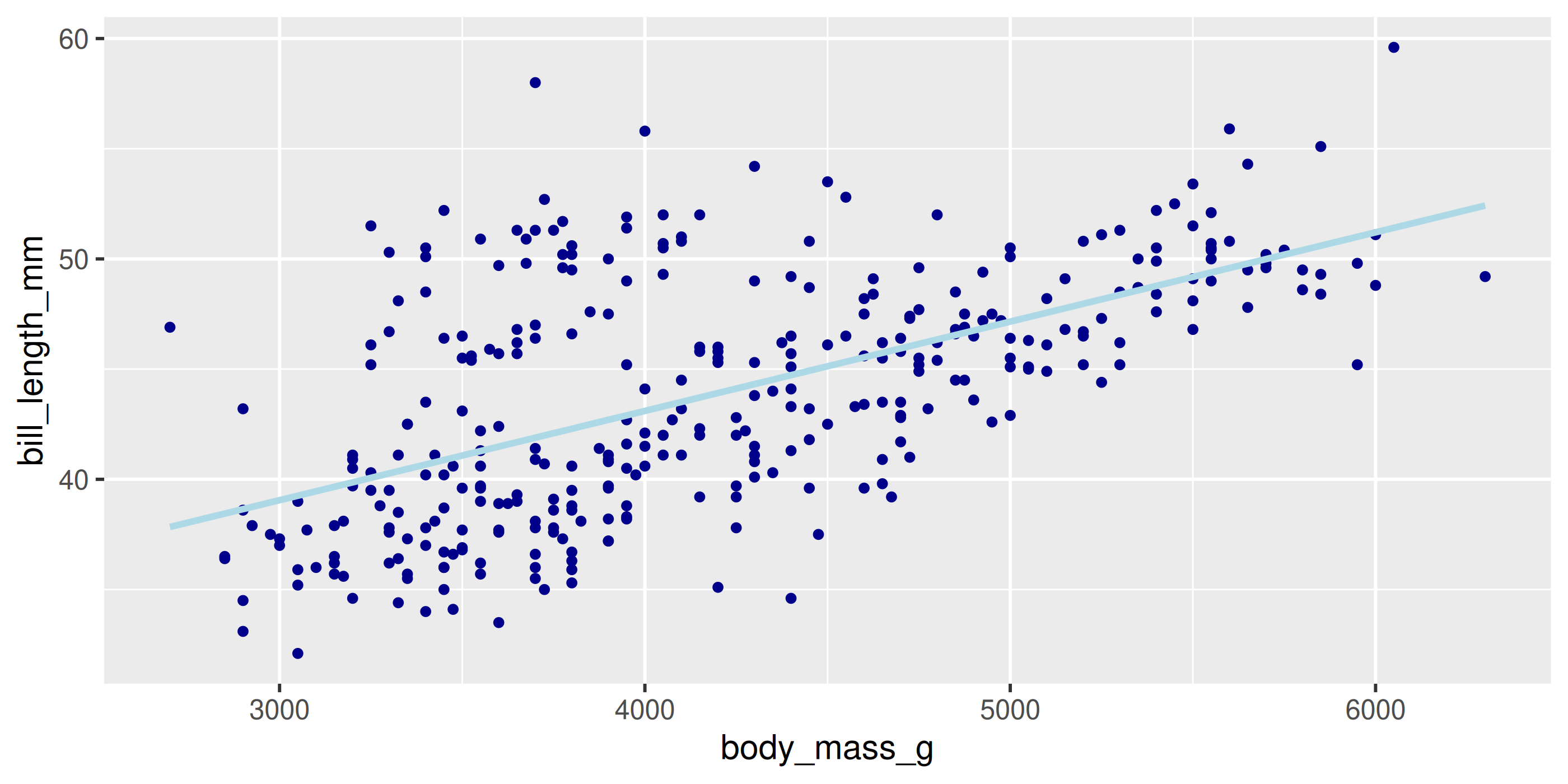
Let’s add a trend line properly
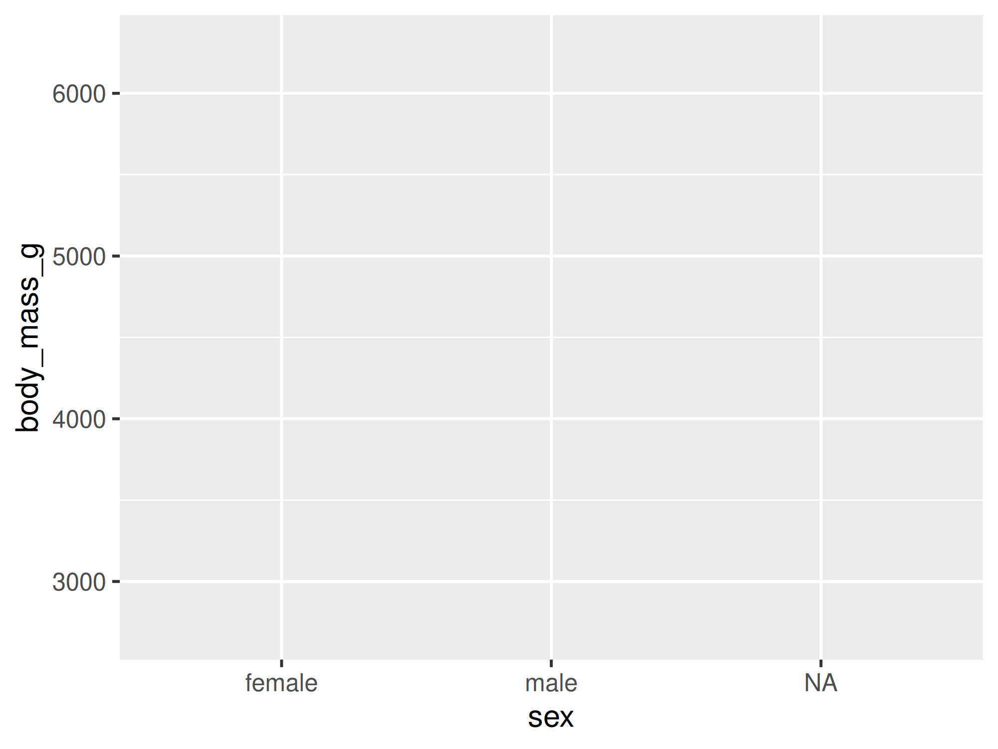
Start with basic plot:

Trendlines / Regression lines
Add the stat_smooth()
lmis for “linear model” (i.e. trendline)- grey ribbon = standard error

Trendlines / Regression lines
Add the stat_smooth()
- remove the grey ribbon
se = FALSE
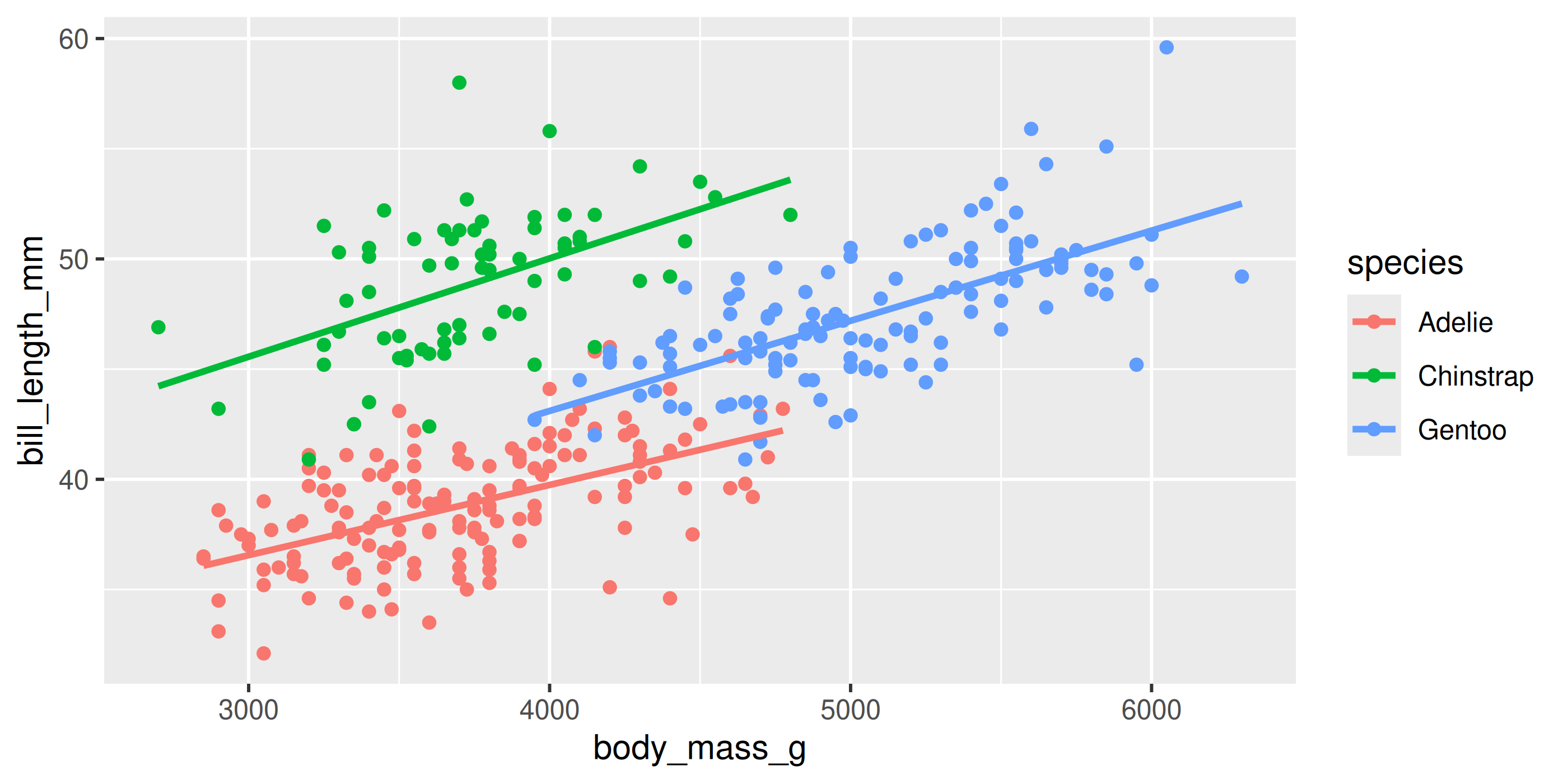
Trendlines / Regression lines
A line for each group
- Specify group (here we use
colourto specifyspecies)
Trendlines / Regression lines
A line for each group
stat_smooth()automatically uses the same grouping
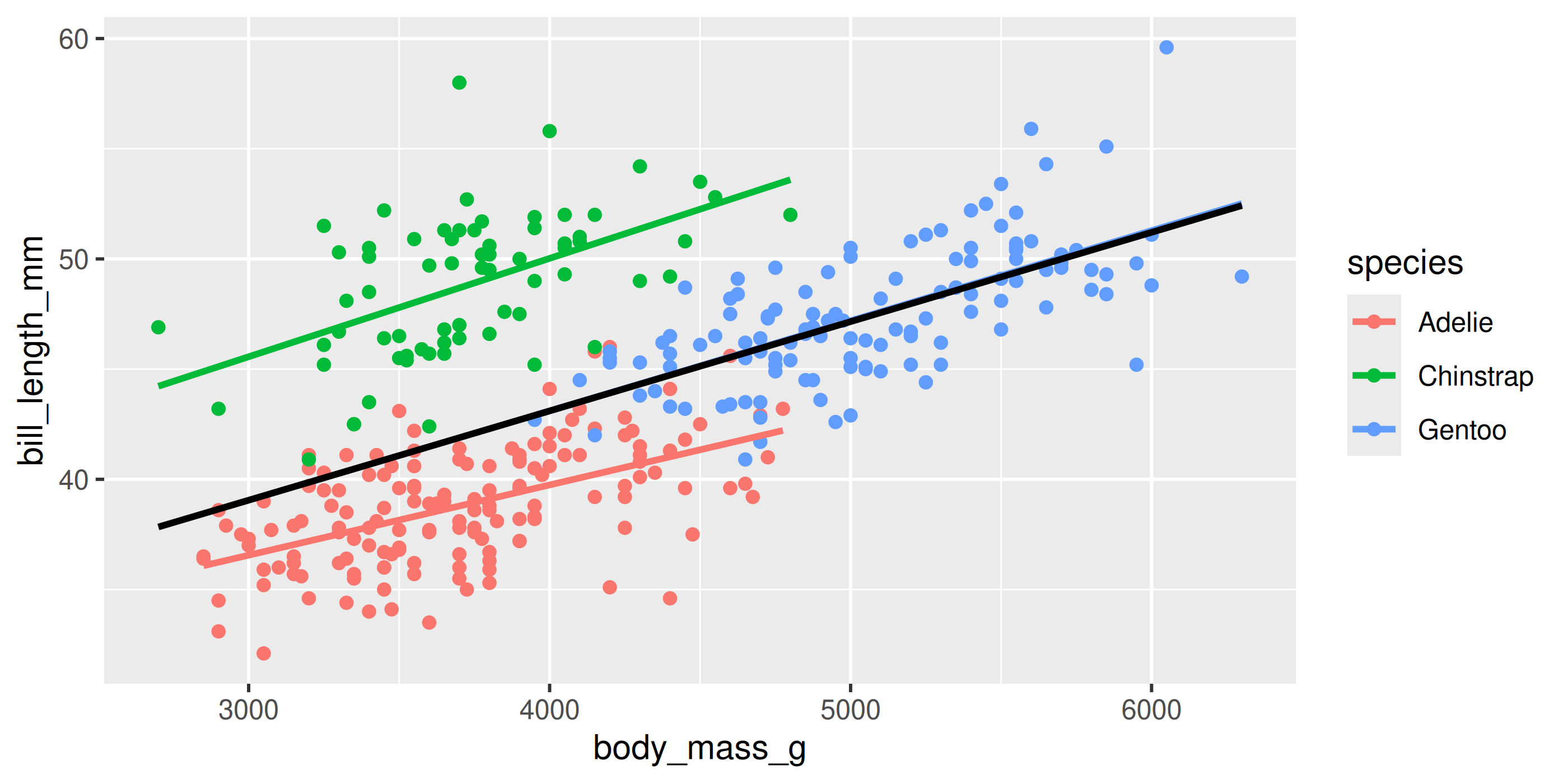
Trendlines / Regression lines
A line for each group AND overall
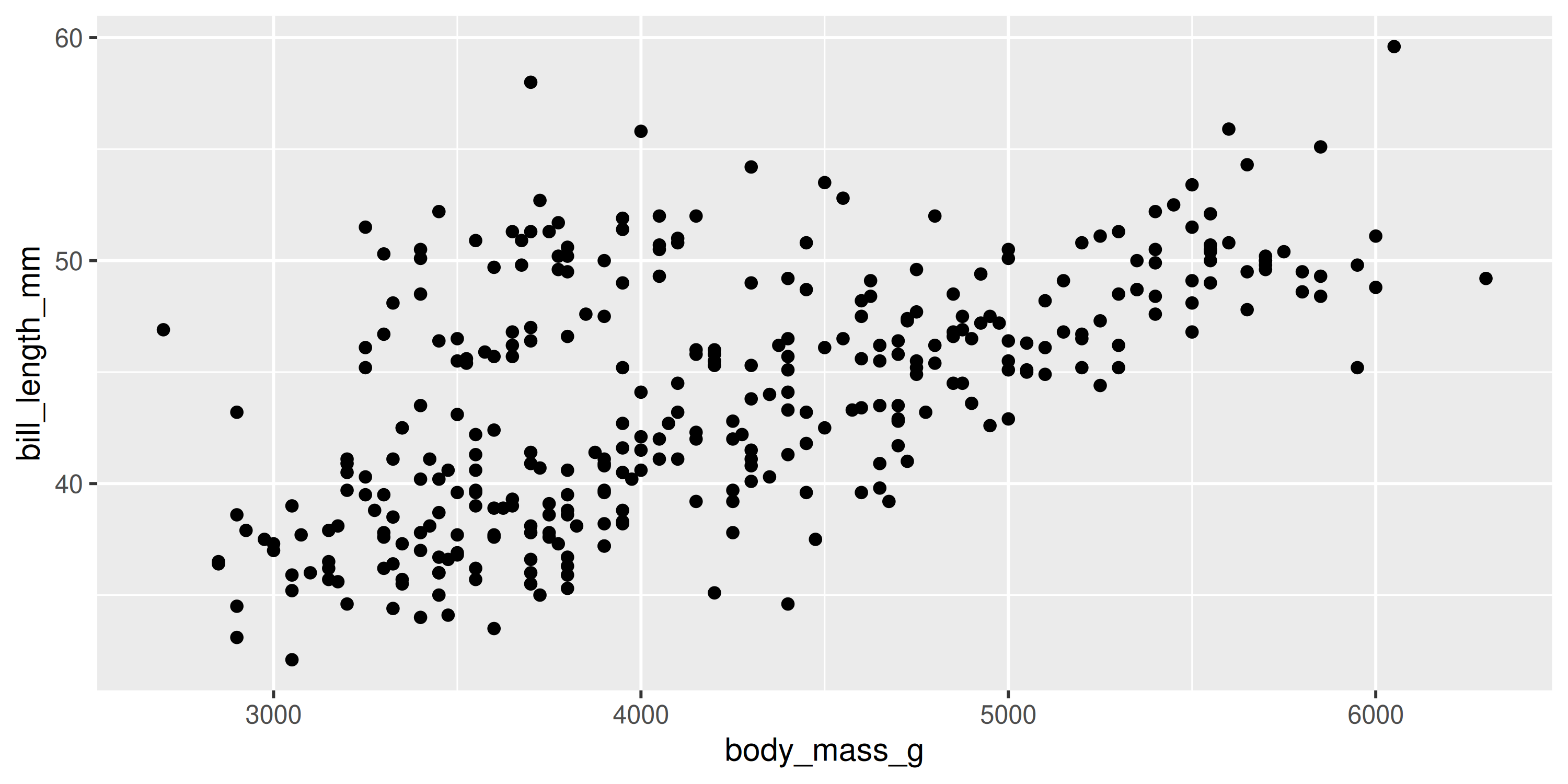
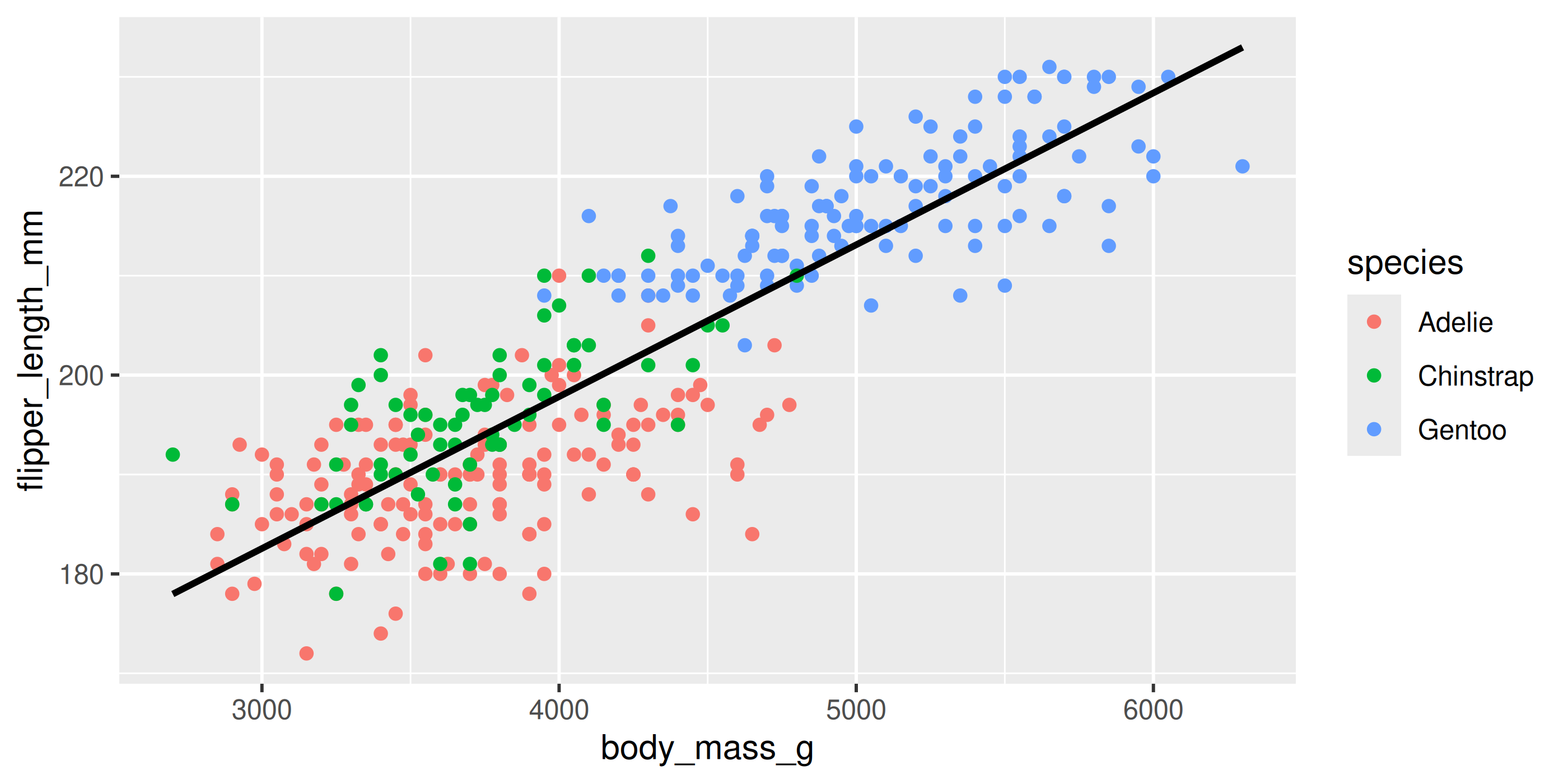
Your Turn: Create this plot
- A scatter plot: Flipper Length by Body Mass grouped by Species
- With a single regression line for the overall trend
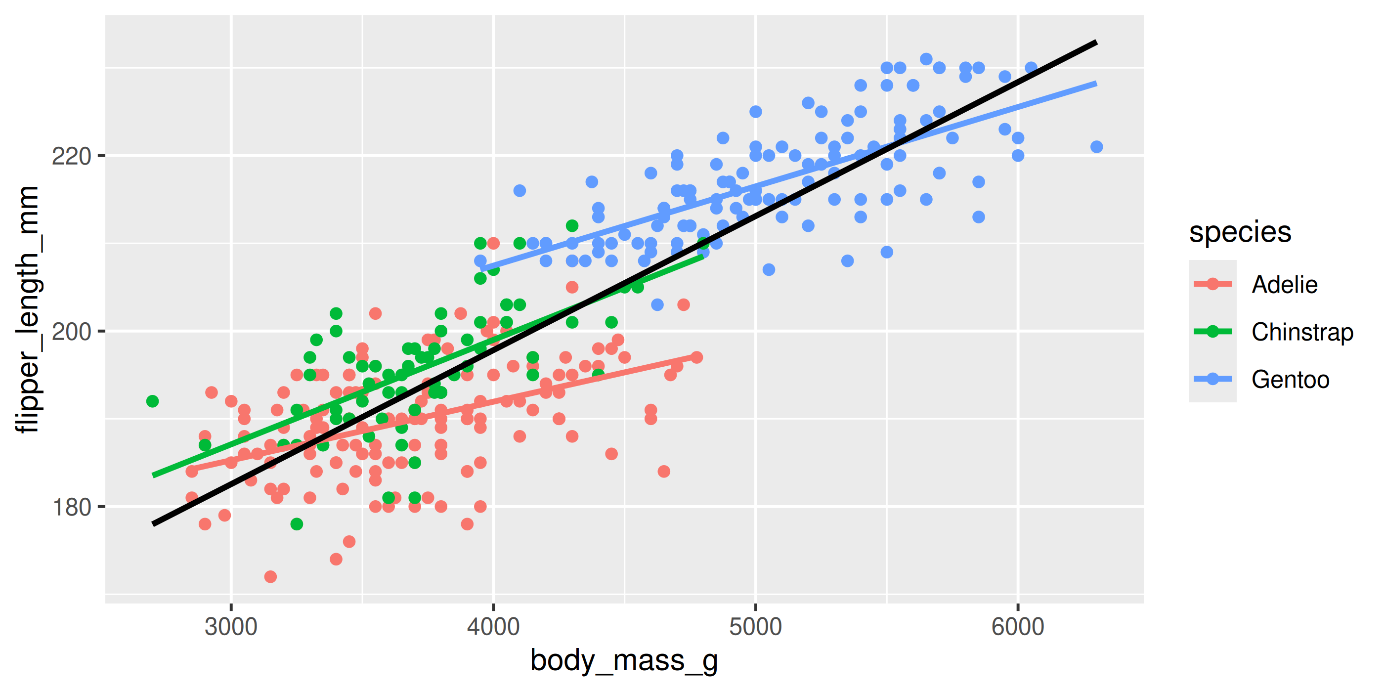
Your Turn: Create this plot
Too Easy?
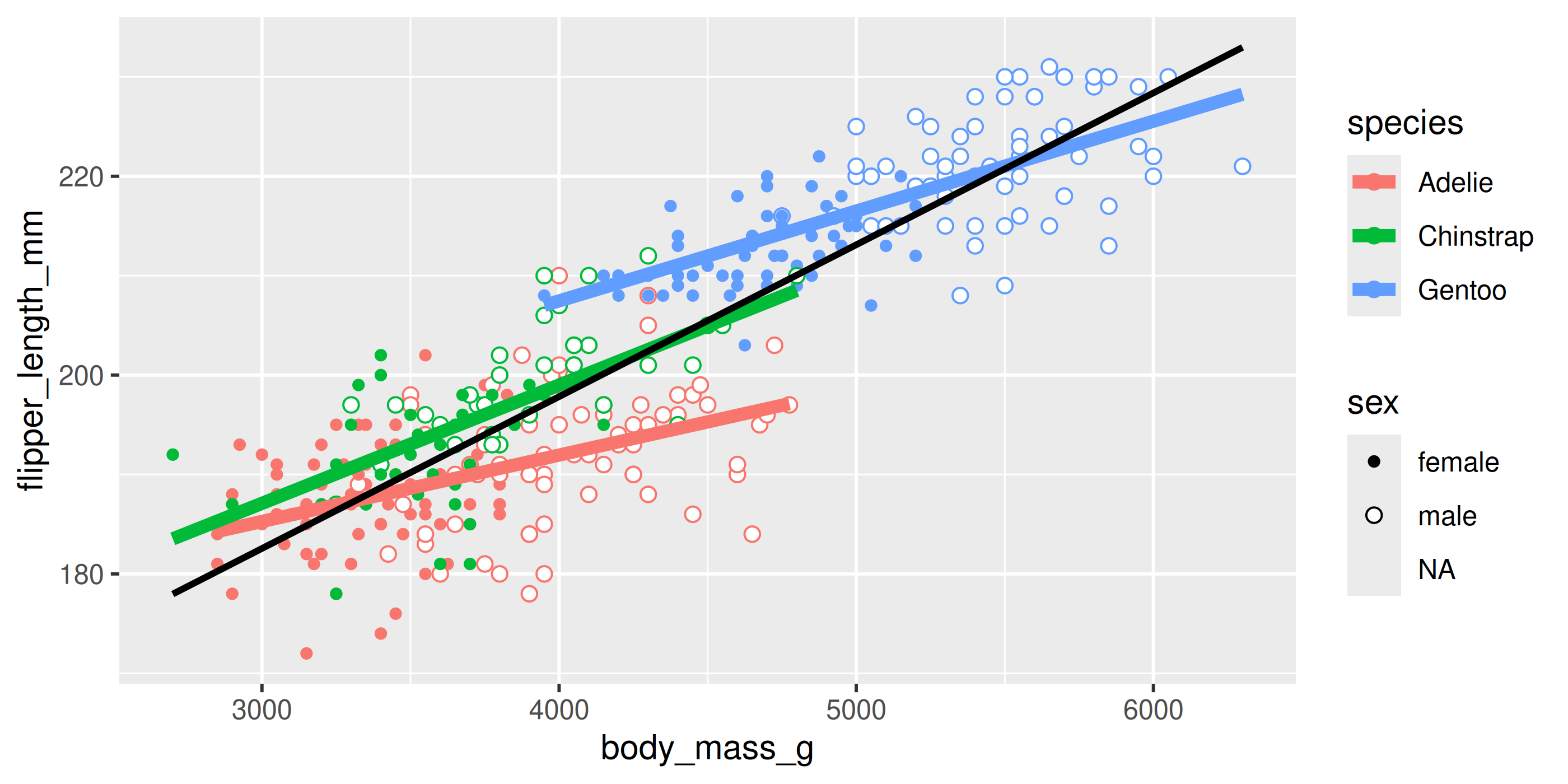
Your Turn: Create this plot
Too Easy?
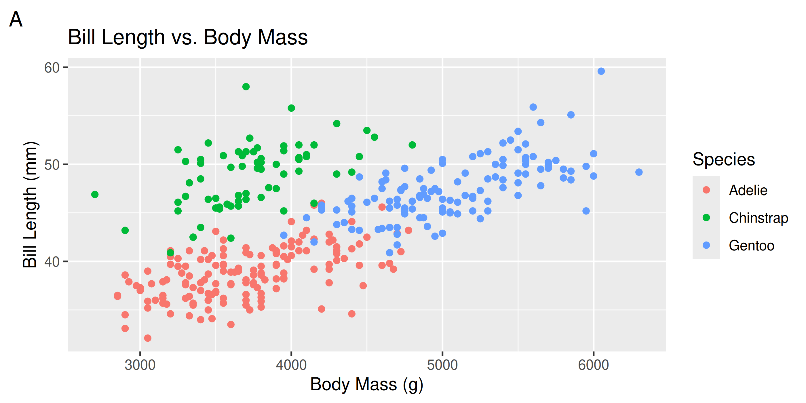
Customizing: Starting plot
Let’s work with this plot

Customizing: Labels
Your Turn: Add proper labels to some of your previous plots
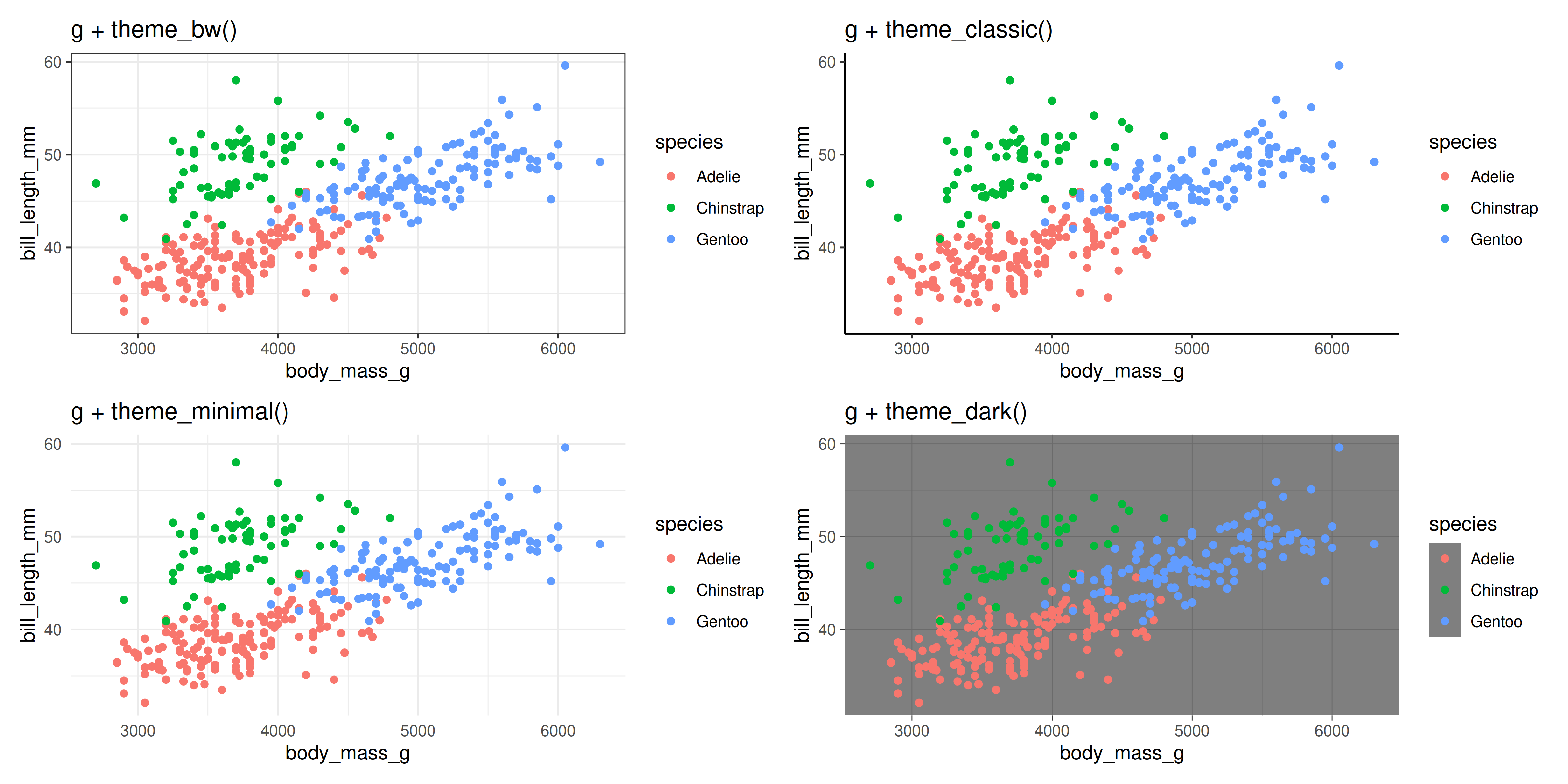
Customizing: Built-in themes
Customizing: Axes
Breaks

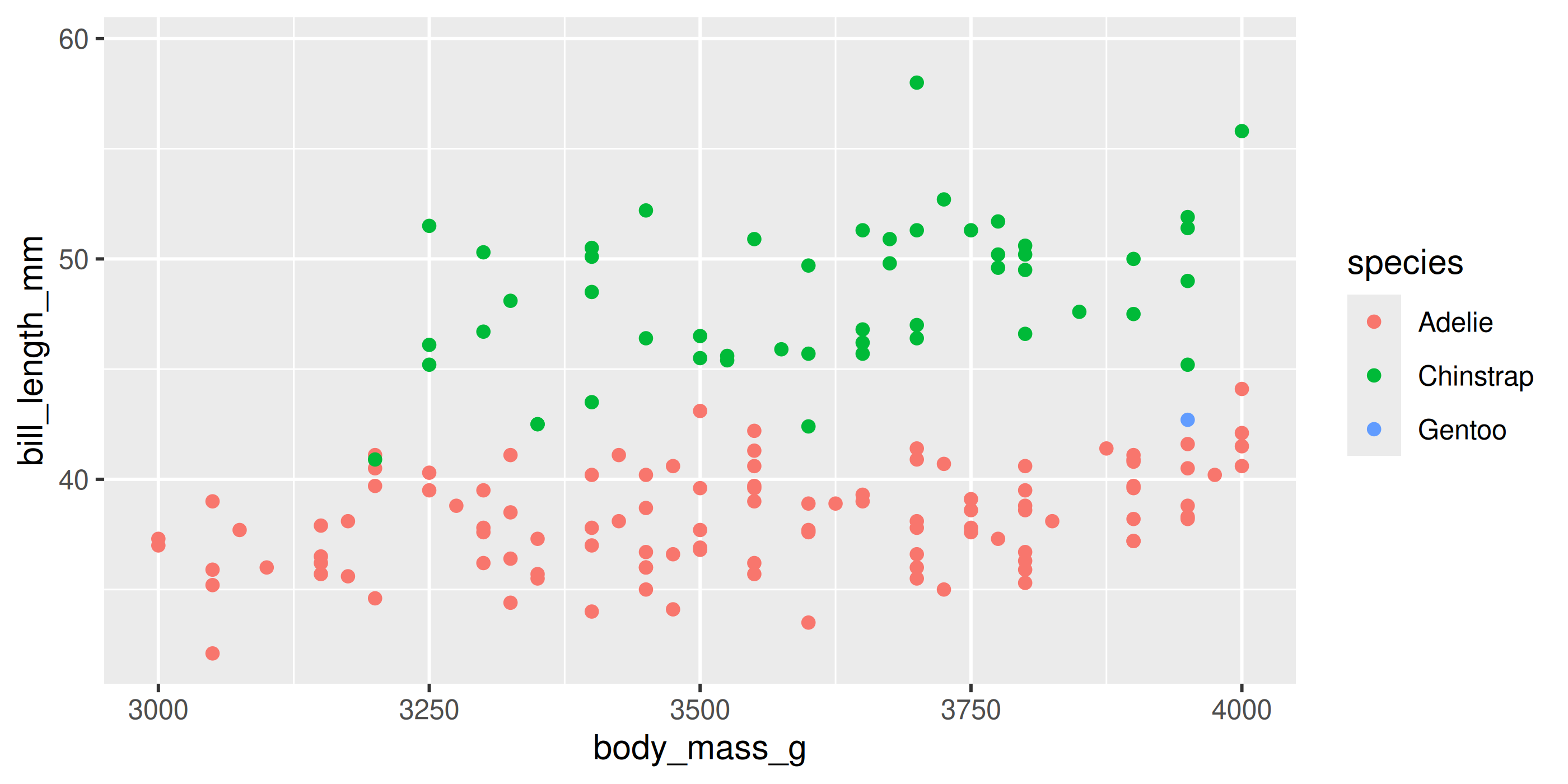
Customizing: Axes
Limits
Customizing: Axes
Space between origin and axis start
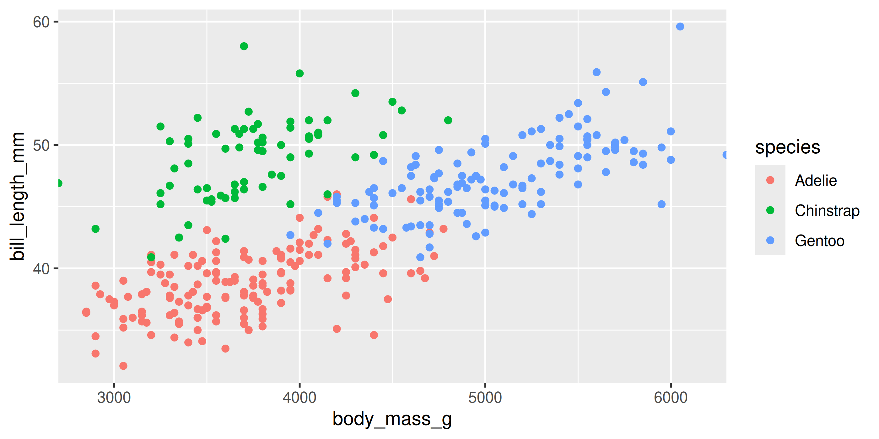
Customizing: Aesthetics
Using scales
scale_ + aesthetic (colour, fill, size, etc.) + type (manual, continuous, datetime, etc.)
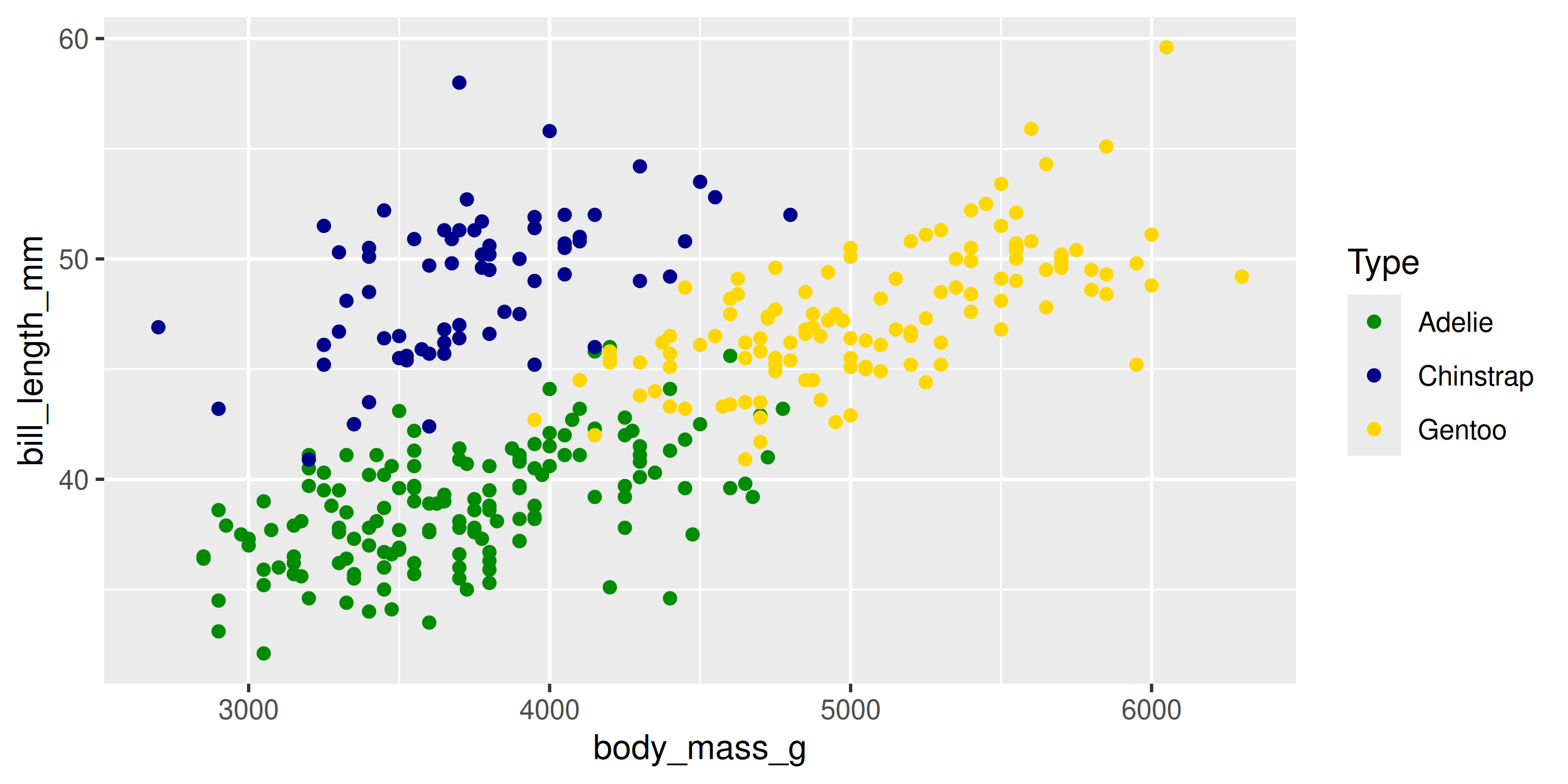
Customizing: Aesthetics
Using scales
Or be very explicit:
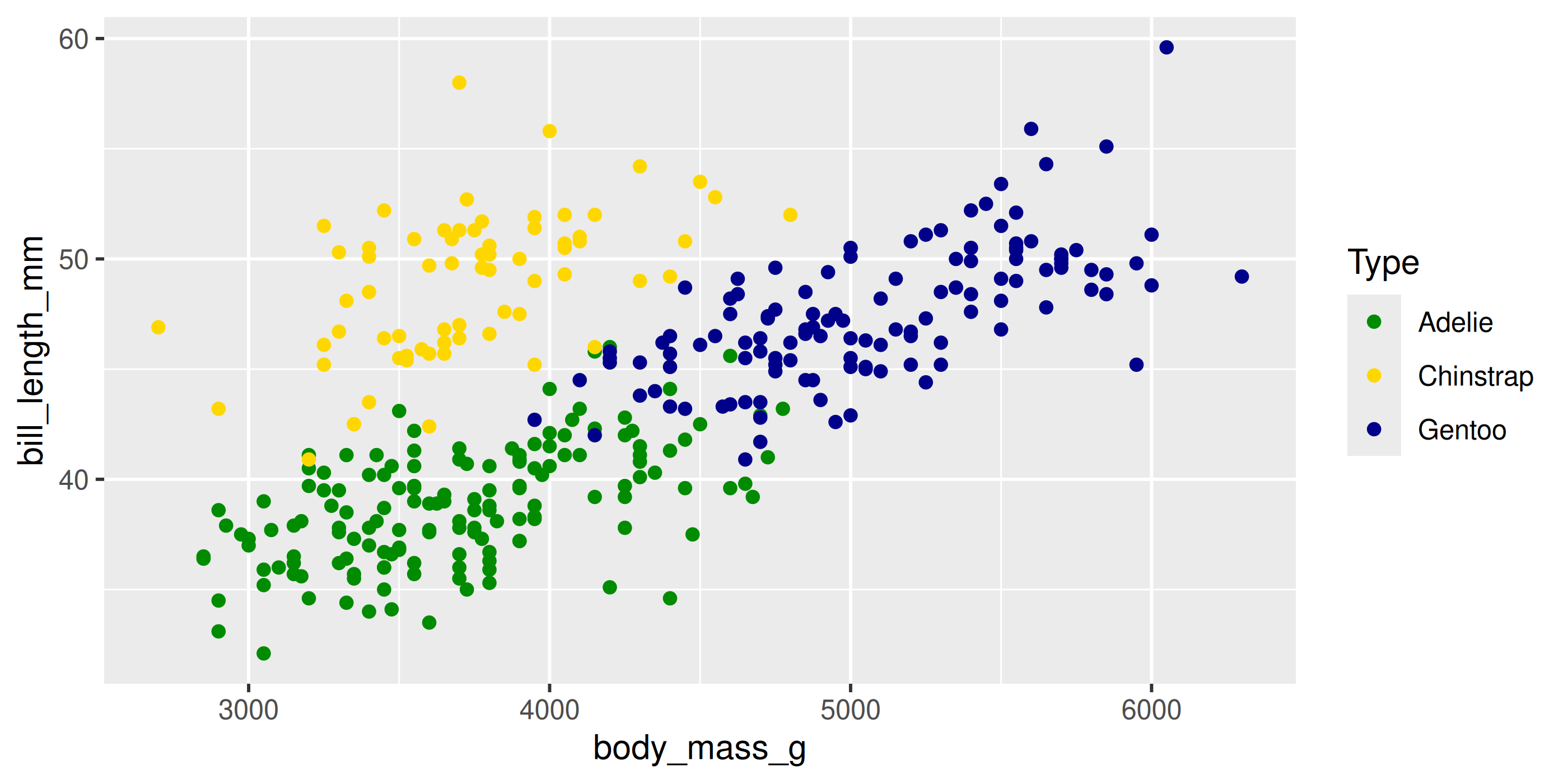
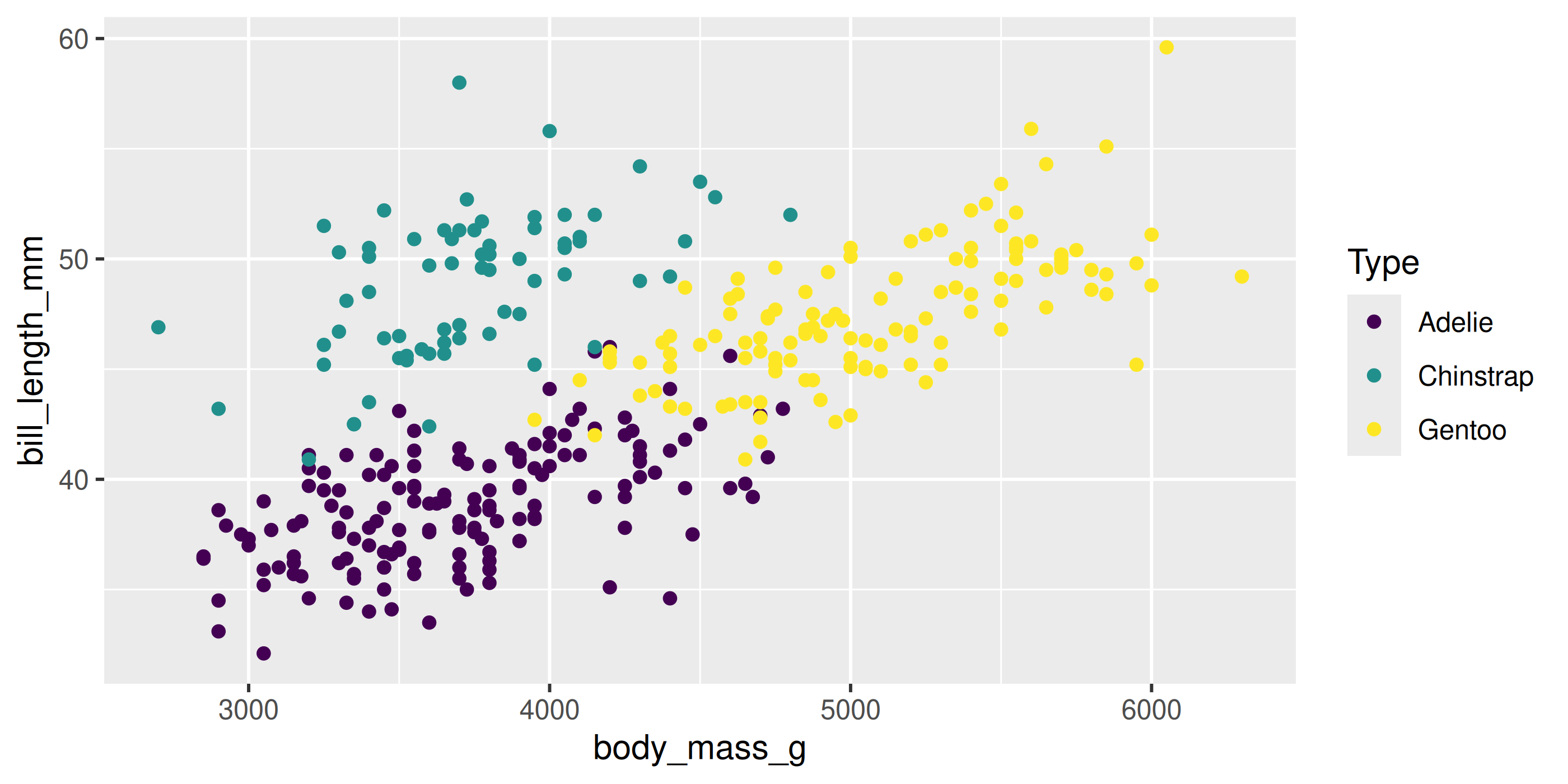
Customizing: Aesthetics
For colours, consider colour-blind-friendly scale
viridis_d for “discrete” data
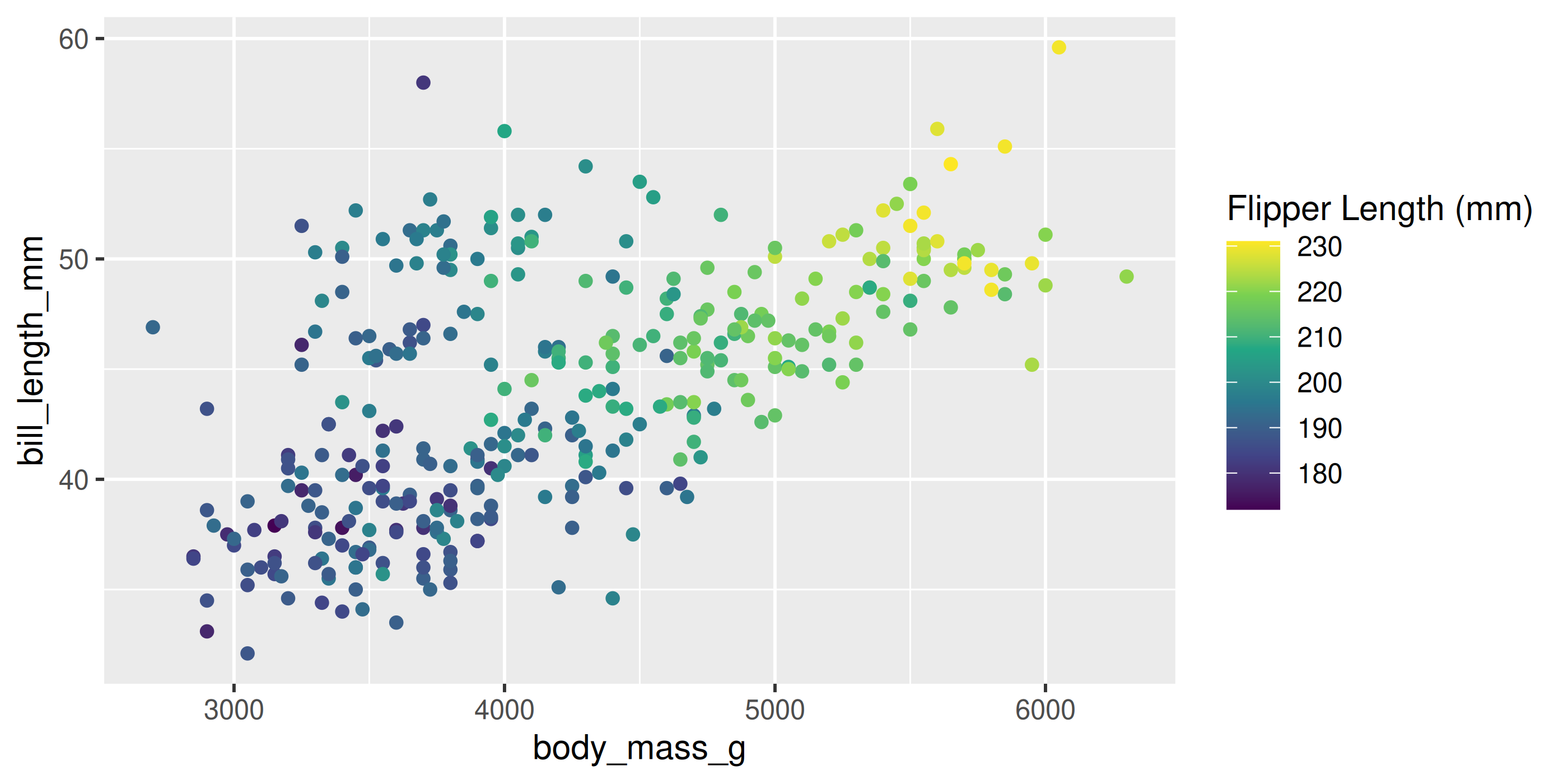
Customizing: Aesthetics
For colours, consider colour-blind-friendly scale
viridis_c for “continuous” data
Customizing: Aesthetics
Forcing
Remove the association between a variable and an aesthetic
Note: When forcing, aesthetic is not inside aes()
Customizing: Legends placement
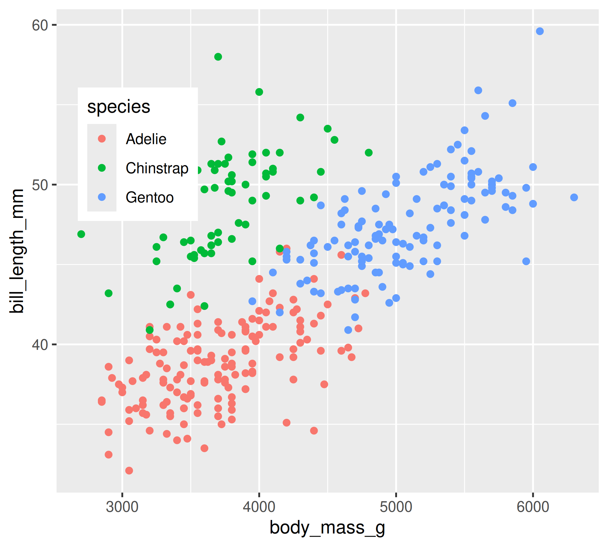
Your Turn: Create this plot

Too Easy?
Play with shape values >20 and fill and colour
Or, create a plot of your own data
Your Turn: Create this plot
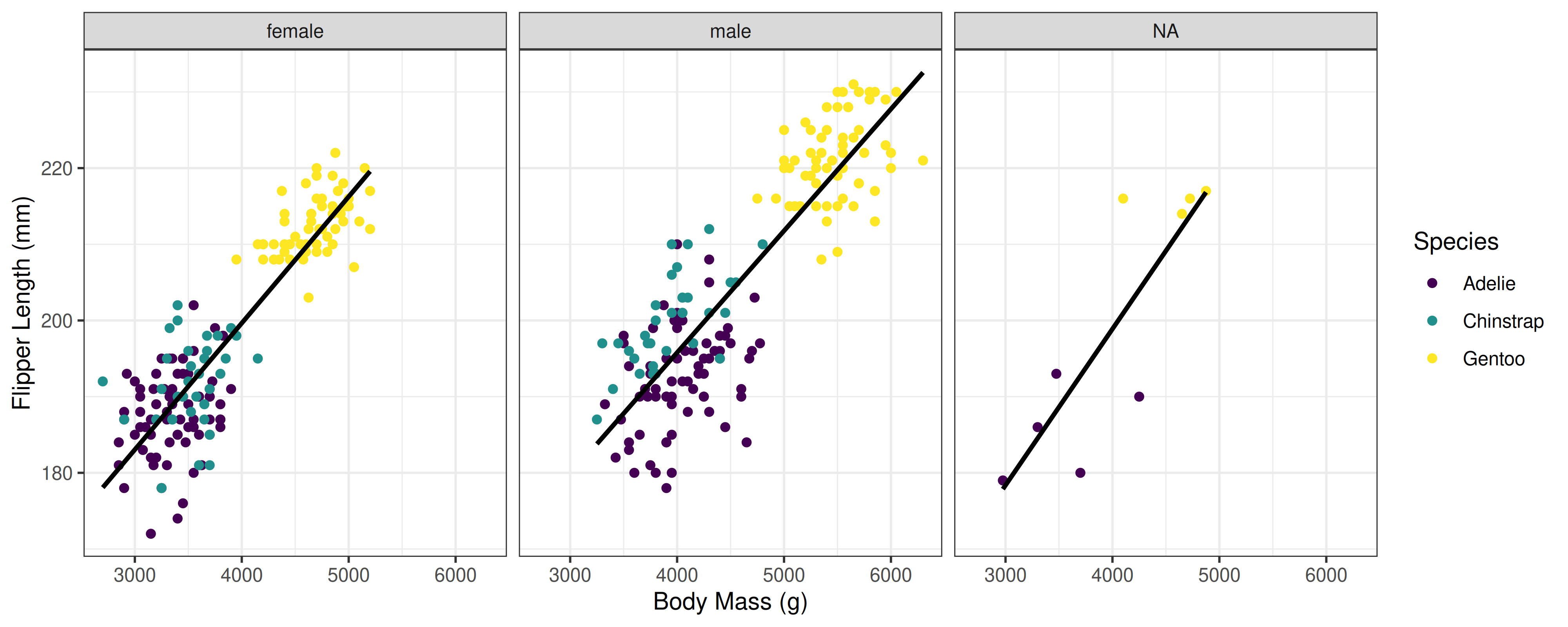
Your Turn: Create this plot
Too easy?
Shape values > 20 are fillable!
ggplot(penguins, aes(x = body_mass_g, y = flipper_length_mm, fill = species)) +
  theme_bw() +
  geom_point(shape = 21) +
  stat_smooth(method = "lm", se = FALSE, colour = "black", fill = NA) +
  scale_fill_viridis_d() +
  facet_wrap(~ sex) +
  labs(x = "Body Mass (g)",
       y = "Flipper Length (mm)",
       colour = "Species")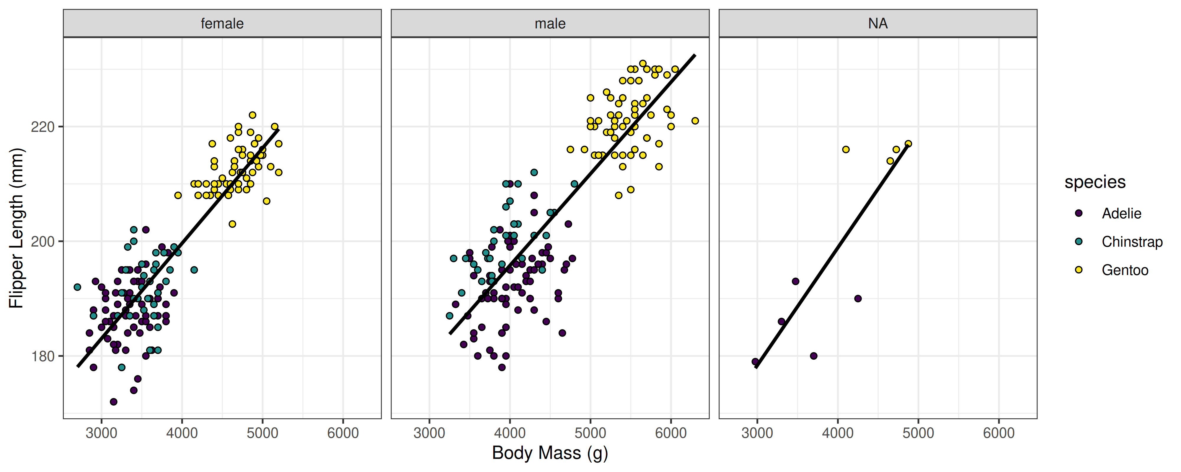
Your Turn: Create this plot
Too easy?
Shape values > 20 are fillable!
Order of operations
Where to put the aes()?
Sometimes it doesn’t matter…


Order of operations
Where to put the aes()?
Sometimes it DOES matter…


Applies to ALL lines in the ggplot
including stat_smooth()
Applies to only the geom_point() in the ggplot
not stat_smooth()
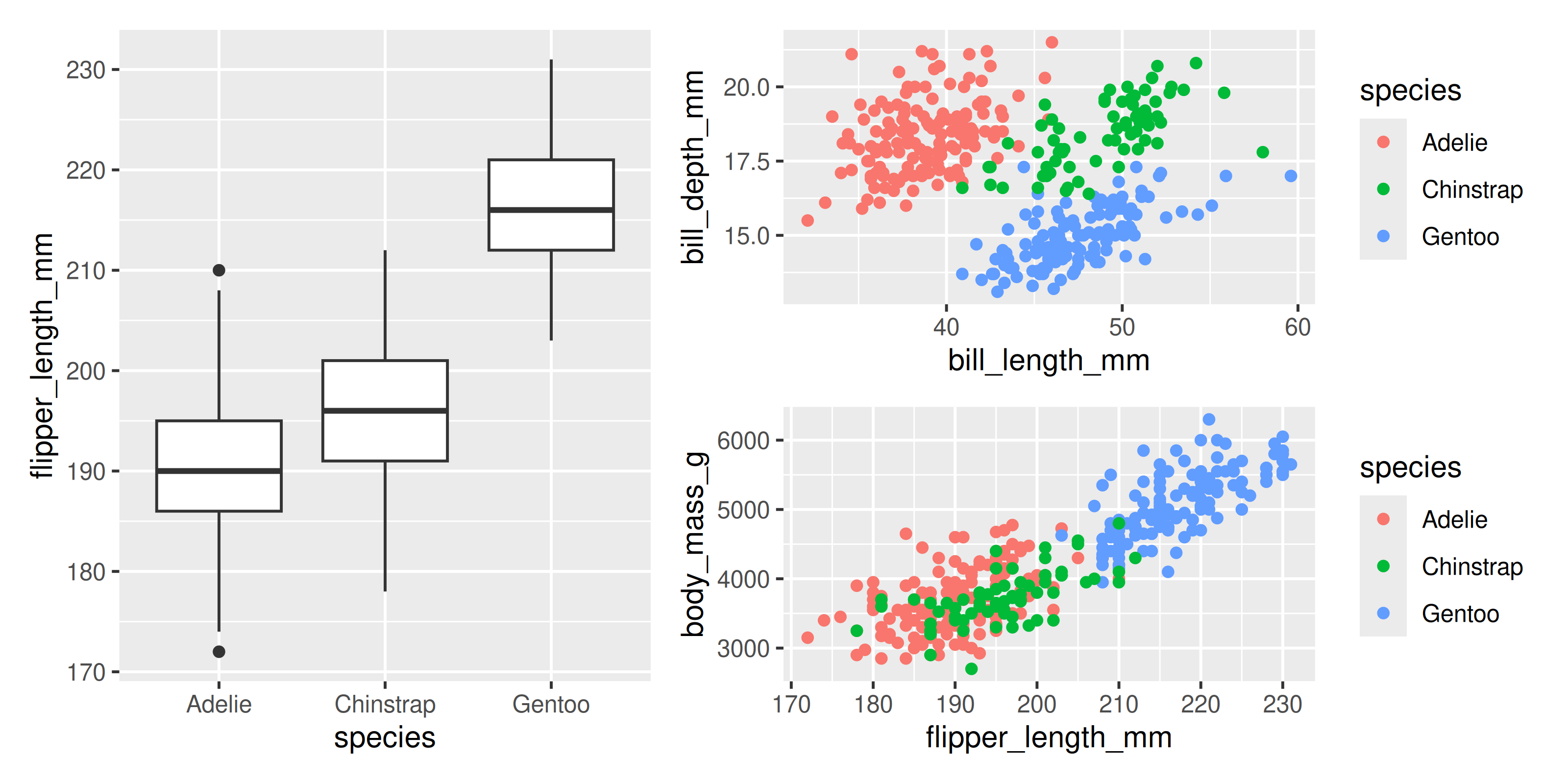
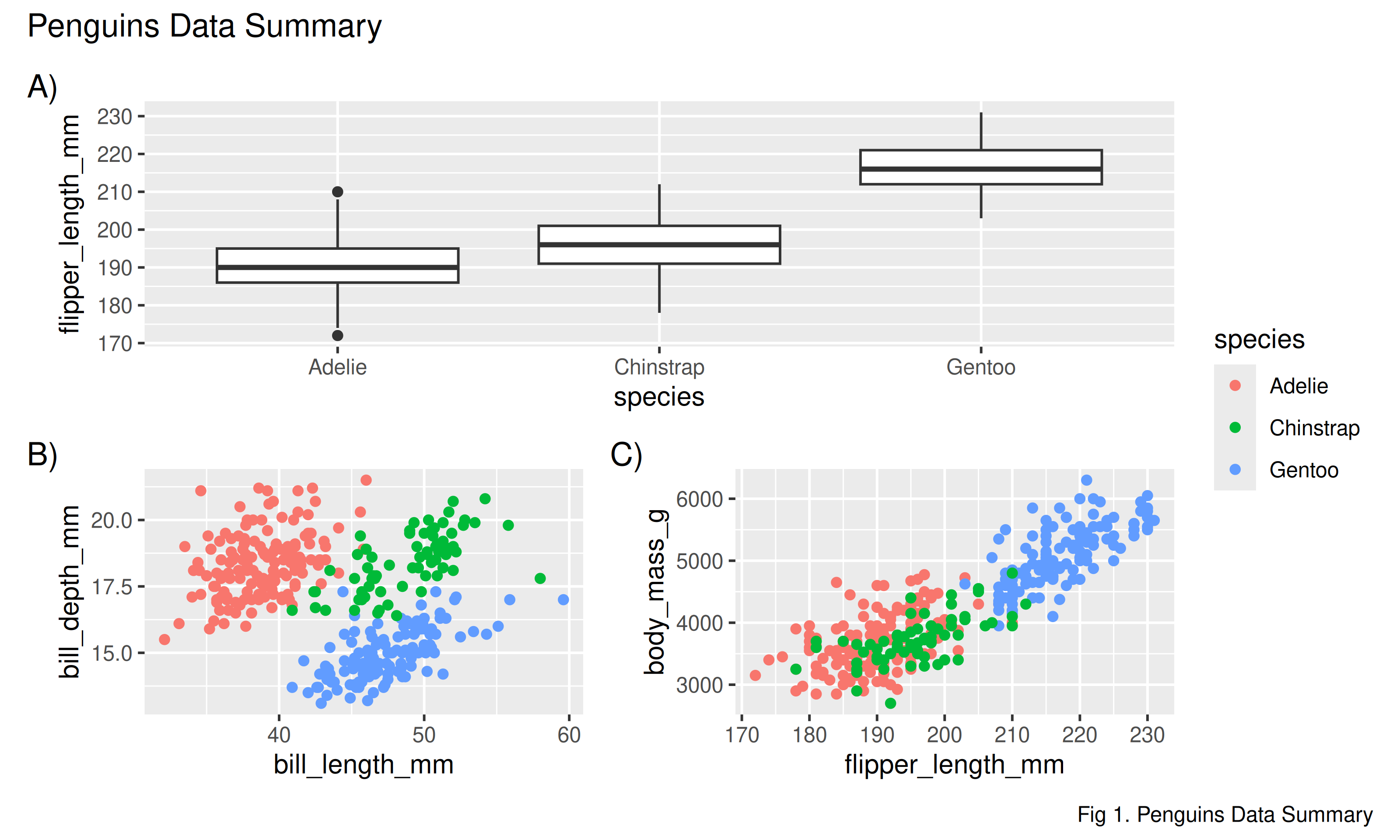
Combining plots with patchwork
![]()
Combining plots with patchwork
Side-by-Side 2 plots
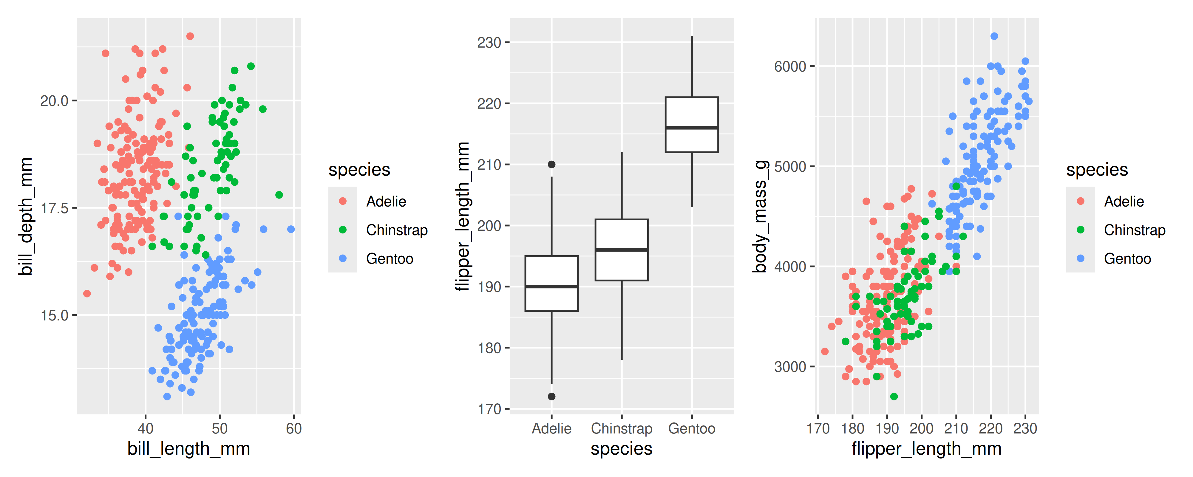
Combining plots with patchwork
Side-by-Side 3 plots
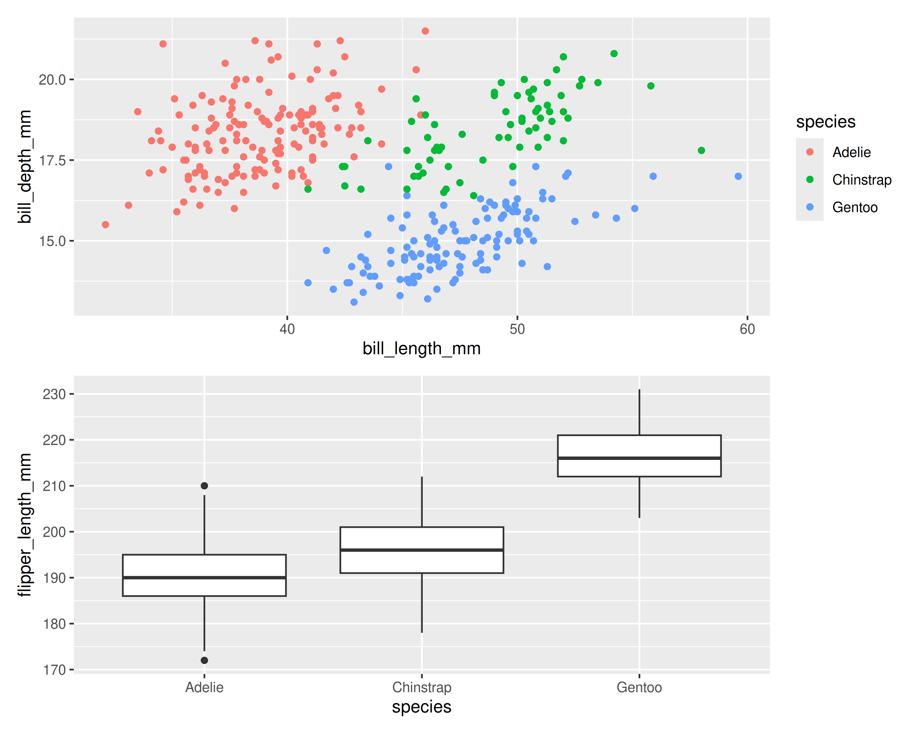
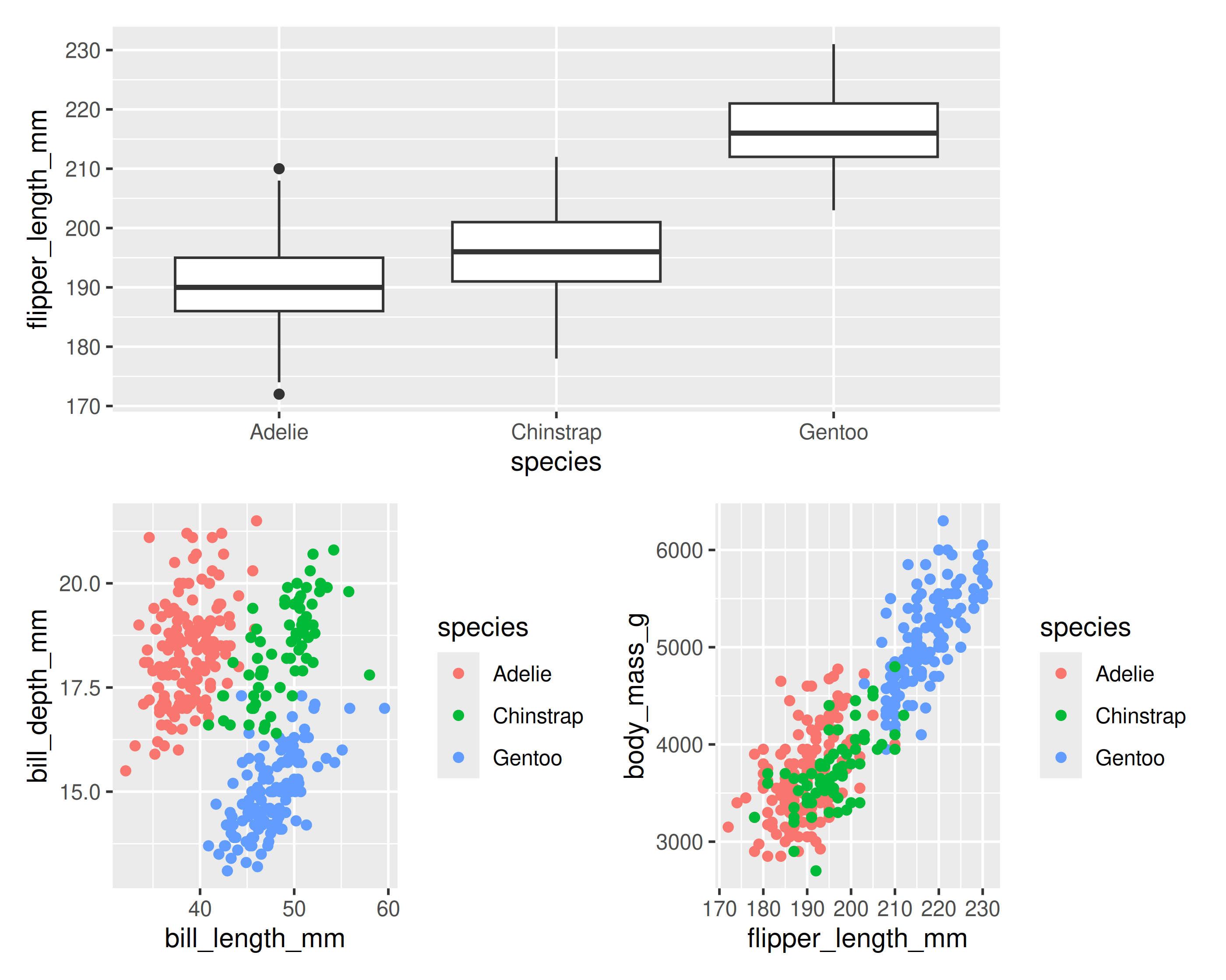
Combining plots with patchwork
Stacked 2 plots
Combining plots with patchwork
More complex arrangements
Combining plots with patchwork
More complex arrangements
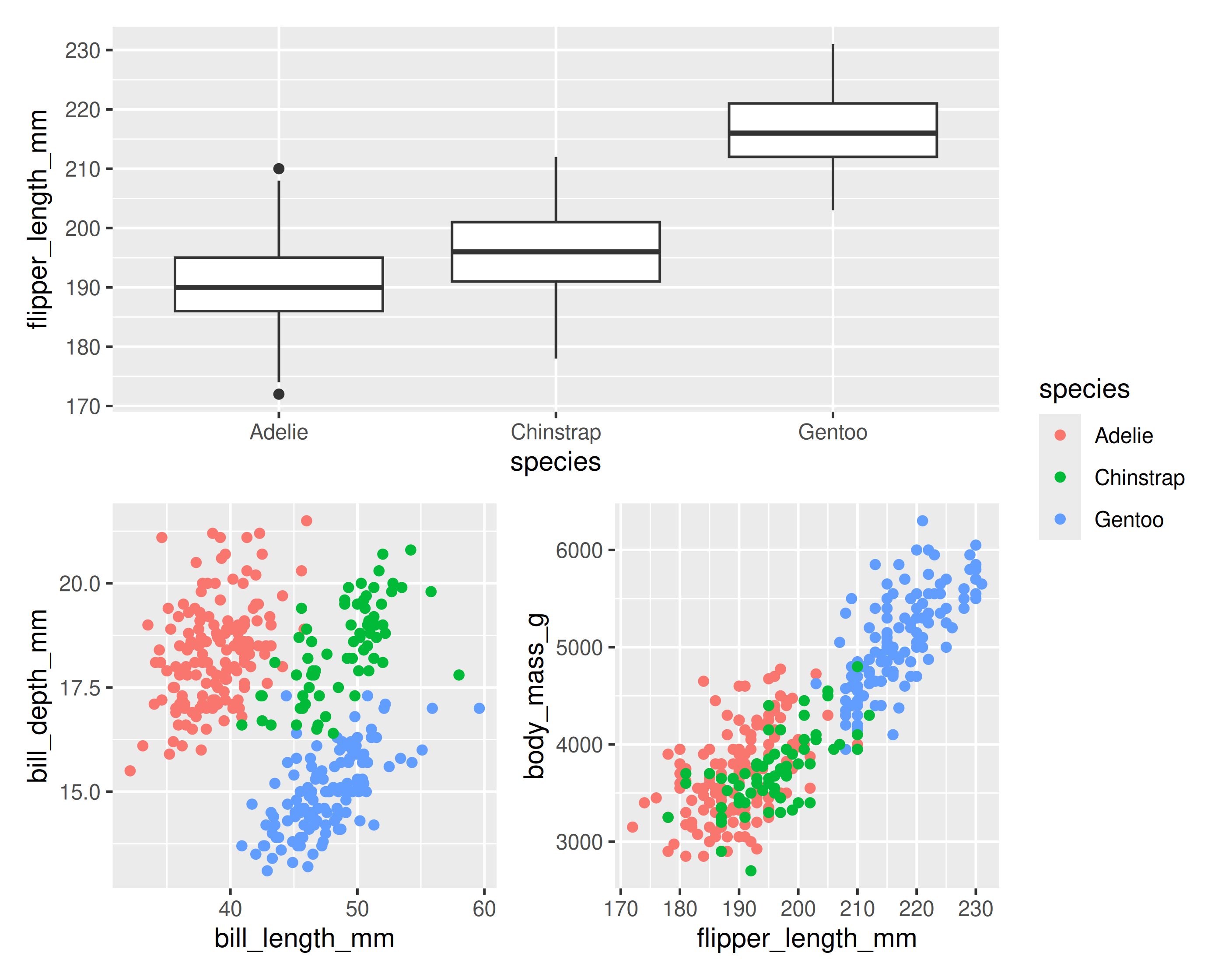
Combining plots with patchwork
“collect” common legends
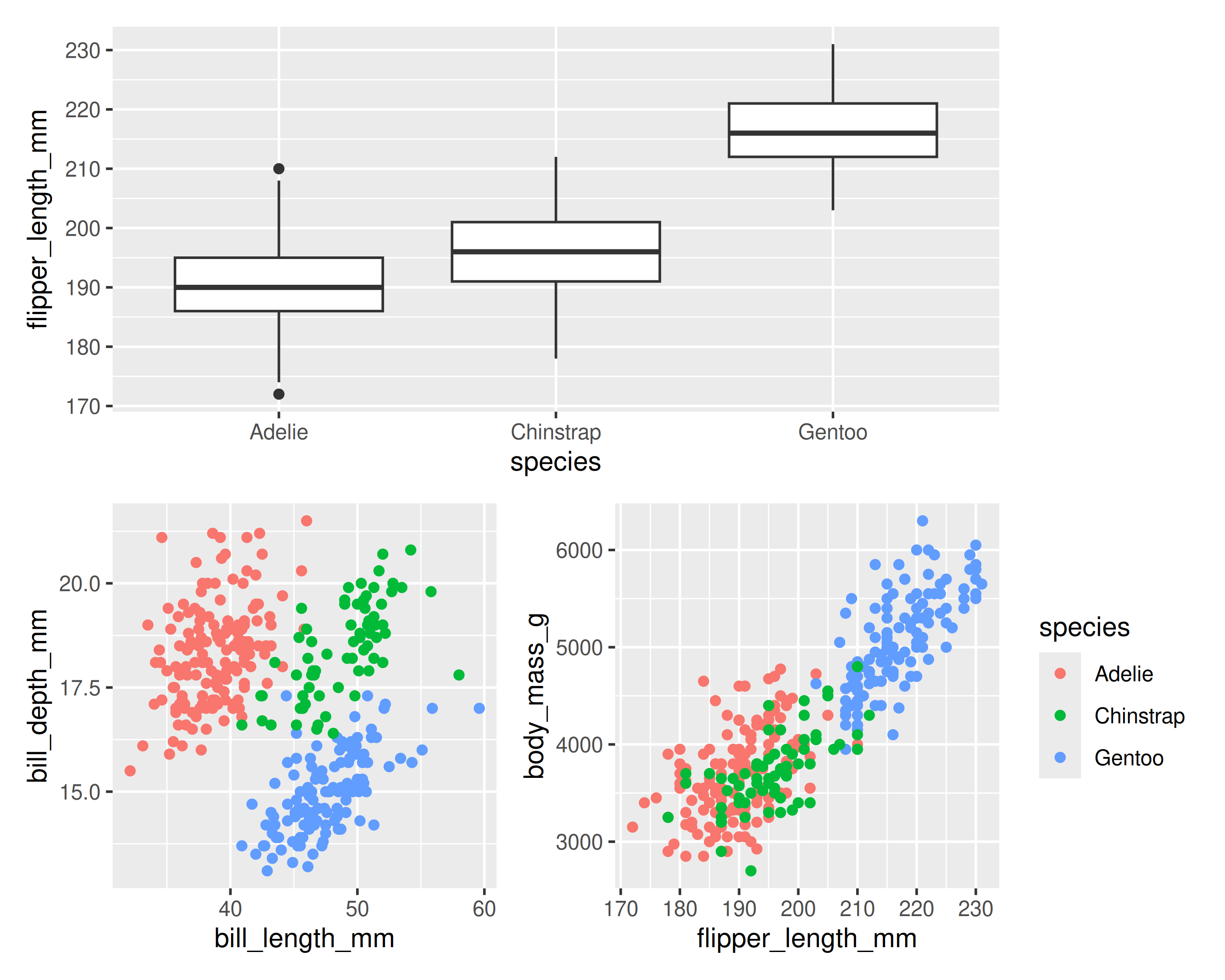
Combining plots with patchwork
“collect” common legends
Combining plots with patchwork
Annotate

Your Turn
Combine any 3 figures Too Easy?
Can you figure out how to collect common axes as well?
Your Turn: Combine plots
Too easy?

Wrapping up: Common mistakes
I get an error regarding an object that can’t be found or aesthetic length?
Either move the aesthetic…
Wrapping up: Common mistakes
I get an error regarding an object that can’t be found or aesthetic length?
Either move the aesthetic…
Or assign it to NULL where it is missing…
