Error: 'weather.csv' does not exist in current working directory ('/home/steffi/Projects/Workshops/workshop-dealing-with-data').Workshop: Dealing with Data in R
Loading & Cleaning Data in R
I know the file exists, why doesn’t R?
steffilazerte
@steffilazerte@fosstodon.org
@steffilazerte
steffilazerte.ca
![]()
Compiled: 2026-02-19
Download the data we’ll use in this workshop
- Create a ‘data’ folder in your RStudio project
- In the “Files” pane click on the folder icon OR
- Navigate to your project folder via your computer’s file browser
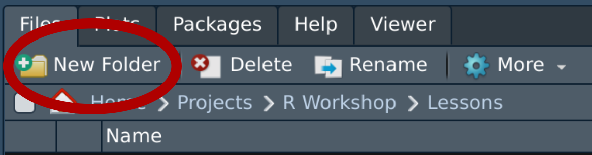
Click on “New Folder”
- Right-click “Save Link As..” and download these files to your data folder
R base vs. tidyverse
R base
- Basic R
- Packages are installed and loaded by default
- Base pipe
|>*
![]()
*We’ll cover pipes soon 😁
tidyverse
- Collection of ‘new’ packages developed by a team closely affiliated with RStudio
- e.g.,
ggplot2,dplyr,tidyr,readr - Packages designed to work well together
- e.g.,
- Use a slightly different syntax
- tidyverse pipe
%>%or base pipe|>*

Useful to know if functions aretidyverse or R base
Data types: What kind of data do you have?
Specific program files
| Type | Extension | R Package | R function |
|---|---|---|---|
| Excel | .xls, .xlsx | readxl* |
read_excel() |
| Open Document | .ods | readODS |
read_ods() |
| SPSS | .sav, .zsav, .por | haven |
read_spss() |
| SAS | .sas7bdat | haven |
read_sas() |
| Stata | .dta | haven |
read_dta() |
| Database Files | .dbf | foreign |
read.dbf() |
Convenient but…
- Can be unreliable
- Can take longer
For files that don’t change, better to save as a *.csv
(Comma-separated-variables file)
 * part of the
 tidyverse
Data types: What kind of data do you have?
General text files
| Type | R base | readr package * |
|---|---|---|
| Comma separated | read.csv() |
read_csv(), read_csv2() |
| Tab separated | read.delim() |
read_tsv() |
| Space separated | read.table() |
read_table() |
| Fixed-width | read.fwf() |
read_fwf() |
 * part of the
 tidyverse
readrpackage especially useful for big data sets (fast!)- Error/warnings from
readrare a bit more helpful
We’ll focus on
readxlpackageread_excel()
readrpackageread_csv(),read_tsv()
Where is my data?
A note on file paths (file locations)
- folders separated by
/ home,steffi,Documents,R Projectsare folderssteffiis inside ofhome,Documentsis inside ofsteffi, etc.mydata.csvis a data file insideR Projectsfolder
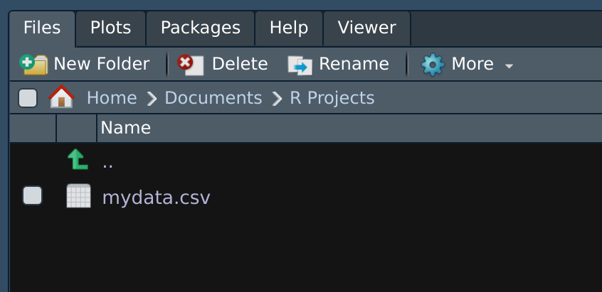
RStudio Files Pane
Your turn: Load some data
Working with 🔗water_cleaned.xlsx
- Load the package
- Read in the Excel file and assign to object
water
Use
head()andtail()functions to look at the data
e.g.,head(water)andtail(water)Click on the
waterobject in your “Environment” pane to look at the whole data set
Your turn: Load some data
# A tibble: 6 × 6
  river       site        element amount temperature  year
  <chr>       <chr>       <chr>    <dbl>       <dbl> <dbl>
1 Grasse      Up stream   Al      0.606       10.9    2019
2 Grasse      Mid stream  Al      0.425        8.68   2020
3 Grasse      Down stream Al      0.194        8.75   2021
4 Oswegatchie Up stream   Al      1            0.791  2022
5 Oswegatchie Mid stream  Al      0.161        9.32   2023
6 Oswegatchie Down stream Al 0.0333 10.6 2019# A tibble: 6 × 6
river site element amount temperature year
<chr> <chr> <chr> <dbl> <dbl> <dbl>
1 Raquette Up stream Zr 0.333 14.0 2023
2 Raquette Mid stream Zr 0.111 7.61 2019
3 Raquette Down stream Zr NA 7.36 2020
4 St. Regis Up stream Zr 0.889 7.94 2021
5 St. Regis Mid stream Zr 0.778 9.28 2022
6 St. Regis Down stream Zr 0.667 10.1 2023
skim() the data
skim() is from skimr
- Are the formats correct?
- numbers (
numeric), - text (
character) - date (
date,POSIXct,datetime) - categories (
factor)
- numbers (
- Are values appropriate?
- Should there be
NAs?
- Should there be
- Are there any typos?
- Number of rows expected?
── Data Summary ────────────────────────
                           Values
Name                       penguins
Number of rows             344
Number of columns          8
_______________________
Column type frequency:
  factor                   3
  numeric                  5
________________________
Group variables            None

── Variable type: factor ───────────────────────────────────────────────────────────────────────────────────────────────────────────────────────────────────────────────────────────────────────────────
  skim_variable n_missing complete_rate ordered n_unique top_counts
1 species               0         1     FALSE          3 Ade: 152, Gen: 124, Chi: 68
2 island                0         1     FALSE          3 Bis: 168, Dre: 124, Tor: 52
3 sex                  11         0.968 FALSE          2 mal: 168, fem: 165

── Variable type: numeric ──────────────────────────────────────────────────────────────────────────────────────────────────────────────────────────────────────────────────────────────────────────────
  skim_variable     n_missing complete_rate   mean      sd     p0    p25    p50    p75   p100 hist
1 bill_length_mm            2         0.994   43.9   5.46    32.1   39.2   44.4   48.5   59.6 ▃▇▇▆▁
2 bill_depth_mm             2         0.994   17.2   1.97    13.1   15.6   17.3   18.7   21.5 ▅▅▇▇▂
3 flipper_length_mm         2         0.994  201.   14.1    172    190    197    213    231   ▂▇▃▅▂
4 body_mass_g               2         0.994 4202.  802.    2700   3550   4050   4750   6300   ▃▇▆▃▂
5 year                      0         1     2008.    0.818 2007   2007   2008   2009   2009   ▇▁▇▁▇
count() categories
count() is from dplyr*
- Check for sample sizes and potential typos in categorical columns
- Assess missing values
 * part of the
 tidyverse
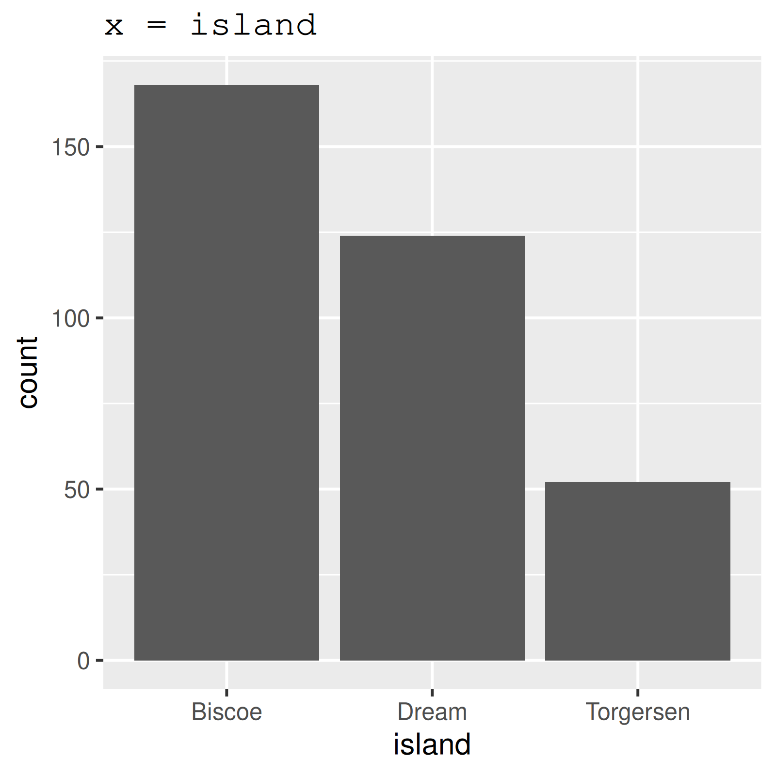
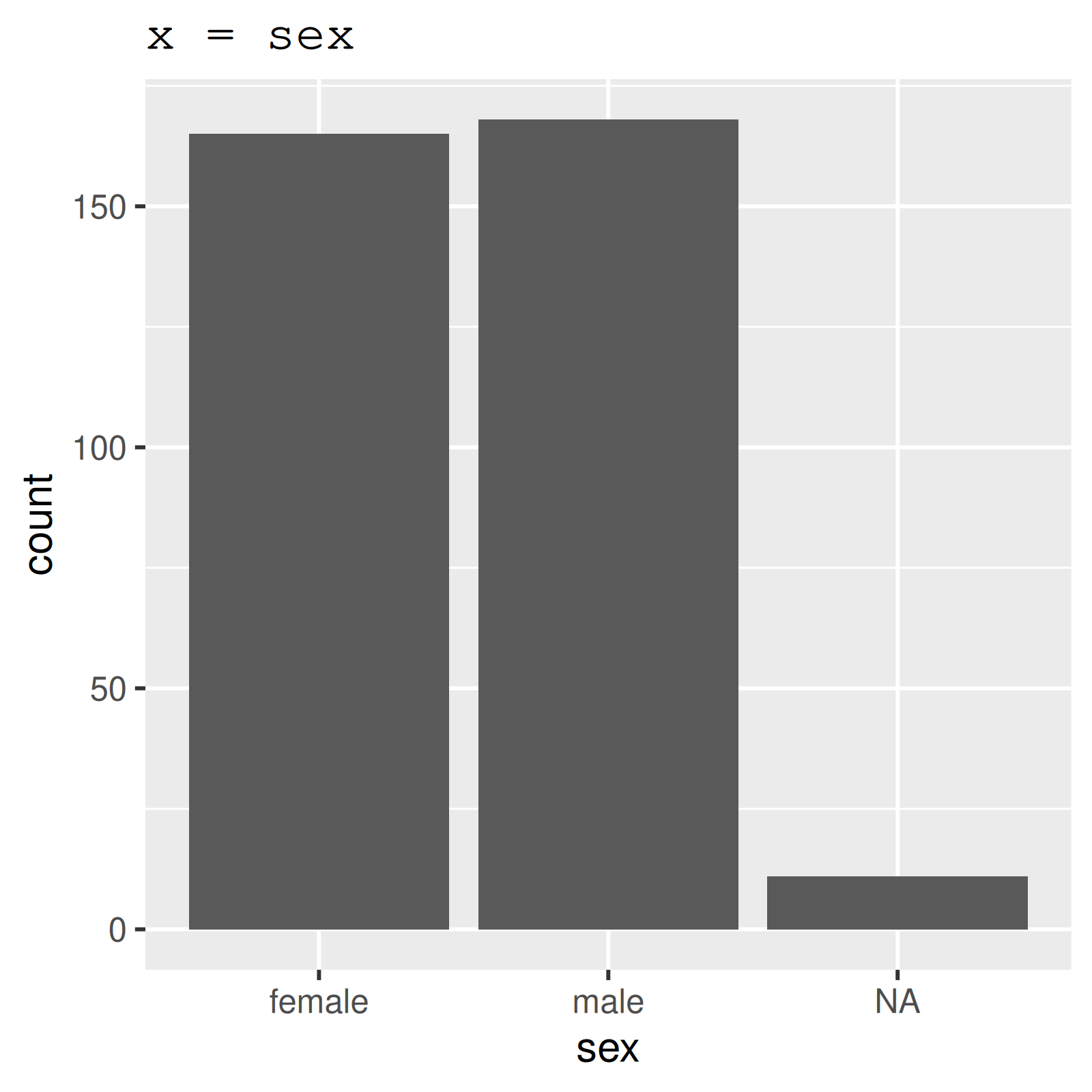
Plot categories

 * part of the
 tidyverse
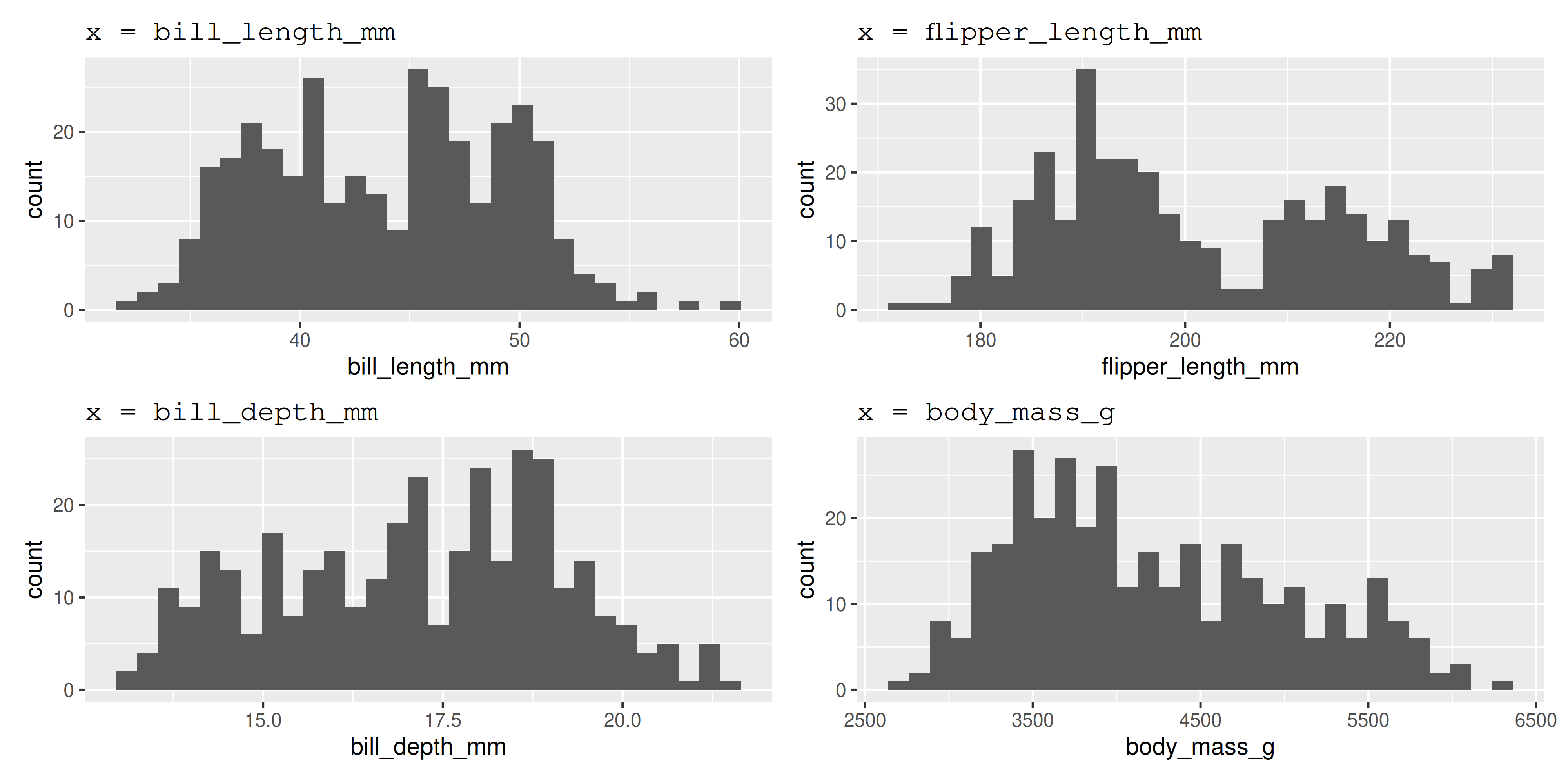
Plot numbers
* part of the tidyverse
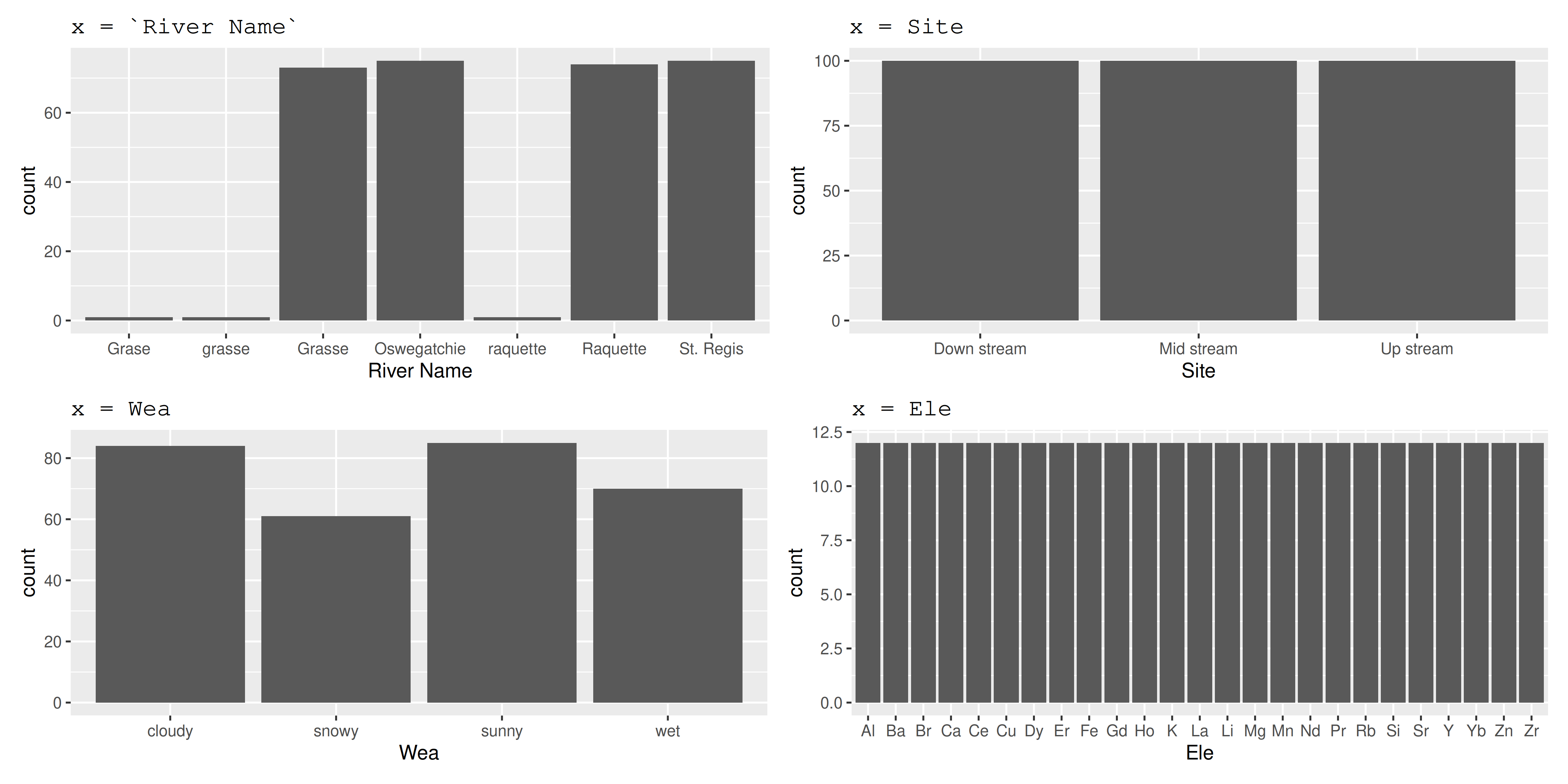
Plot categories
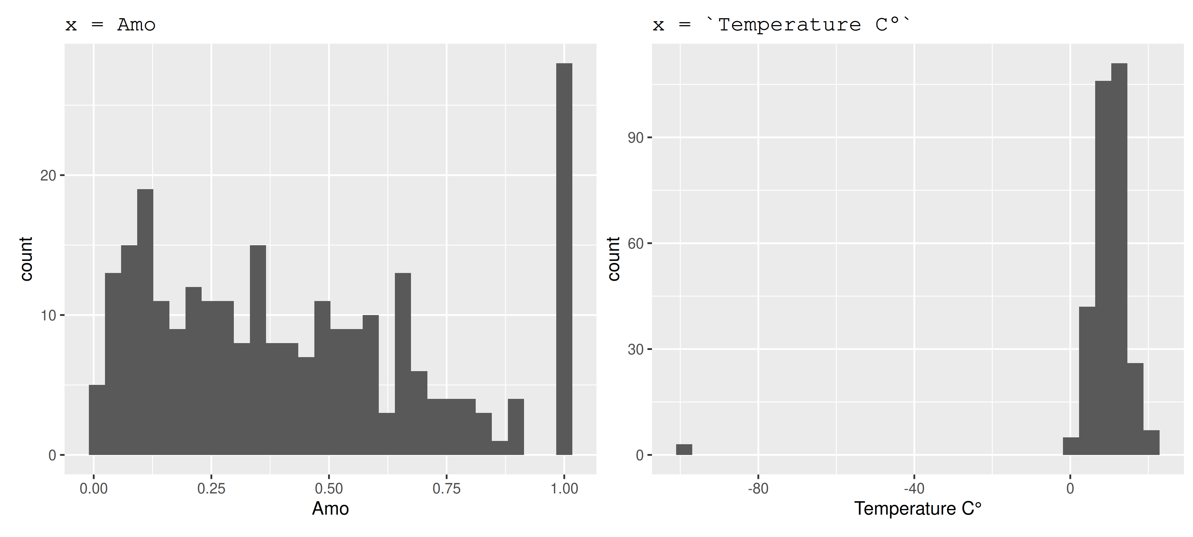
Plot numbers
Cleaning column names
clean_names() is from janitor*
* not part of the tidyverse but tidyverse-orientated
# A tibble: 300 × 7
river_name site ele amo temperature_c year wea
<chr> <chr> <chr> <dbl> <dbl> <dbl> <chr>
1 Grasse Up stream Al 0.606 10.9 2019 snowy
2 Grasse Mid stream Al 0.425 8.68 2020 cloudy
3 Grase Down stream Al 0.194 8.75 2021 cloudy
4 Oswegatchie Up stream Al 1 0.791 2022 sunny
5 Oswegatchie Mid stream Al 0.161 9.32 2023 snowy
6 Oswegatchie Down stream Al 0.0333 10.6 2019 wet
7 Raquette Up stream Al 0.292 4.01 2020 snowy
8 Raquette Mid stream Al 0.0389 5.96 2021 sunny
9 Raquette Down stream Al NA 6.21 2022 cloudy
10 St. Regis Up stream Al 0.681 8.02 2023 wet
# ℹ 290 more rows
Side Note: Naming conventions

Side Note: Naming conventions
Cleaning column names
rename() is from dplyr*
rename() columns
# A tibble: 300 × 7
river_name site element amount temperature year wea
<chr> <chr> <chr> <dbl> <dbl> <dbl> <chr>
1 Grasse Up stream Al 0.606 10.9 2019 snowy
2 Grasse Mid stream Al 0.425 8.68 2020 cloudy
3 Grase Down stream Al 0.194 8.75 2021 cloudy
4 Oswegatchie Up stream Al 1 0.791 2022 sunny
5 Oswegatchie Mid stream Al 0.161 9.32 2023 snowy
6 Oswegatchie Down stream Al 0.0333 10.6 2019 wet
7 Raquette Up stream Al 0.292 4.01 2020 snowy
8 Raquette Mid stream Al 0.0389 5.96 2021 sunny
9 Raquette Down stream Al NA 6.21 2022 cloudy
10 St. Regis Up stream Al 0.681 8.02 2023 wet
# ℹ 290 more rows * part of the tidyverse
Subsetting columns
select() is from dplyr*
select() columns you want
* part of the tidyverse
OR, unselect() columns you don’t want
# A tibble: 300 × 6
river_name site element amount temperature year
<chr> <chr> <chr> <dbl> <dbl> <dbl>
1 Grasse Up stream Al 0.606 10.9 2019
2 Grasse Mid stream Al 0.425 8.68 2020
3 Grase Down stream Al 0.194 8.75 2021
4 Oswegatchie Up stream Al 1 0.791 2022
5 Oswegatchie Mid stream Al 0.161 9.32 2023
6 Oswegatchie Down stream Al 0.0333 10.6 2019
7 Raquette Up stream Al 0.292 4.01 2020
8 Raquette Mid stream Al 0.0389 5.96 2021
9 Raquette Down stream Al NA 6.21 2022
10 St. Regis Up stream Al 0.681 8.02 2023
# ℹ 290 more rowsFixing typos
if_else() and mutate() from dplyr package*
if_else() tests for a condition, and returns one value if FALSE and another if TRUE
* part of the tidyverse
Iterative process
- Make some corrections
- Check the data
- Make some more corrections (either add to or modify existing code)
tidyverse functions
rename(), select(), mutate()
tidyversefunctions always start with the data, followed by other arguments- you can reference any column from ‘data’
rename()changes column namesselect()chooses columns to keep or to remove (with-)mutate()changes column contents
Why use tidyverse functions?
Pipes! |>* Allow you to string commands together
Instead of:
water <- read_csv("data/water_raw.csv")
water <- clean_names(water)
water <- rename(water, element = ele, amount = amo, temperature = temperature_c)
water <- select(water, -wea)
water <- mutate(water,
river_name = case_when(river_name %in% c("Grase", "grasse") ~ "Grasse",
river_name == "raquette" ~ "Raquette",
TRUE ~ river_name))* |> is the base pipe, %>% is the tidyverse pipe, you can use either
Play around
Take a moment to play with this code in your console
Convert this:
water <- read_csv("data/water_raw.csv")
water <- clean_names(water)
water <- rename(water, element = ele, amount = amo, temperature = temperature_c)
water <- select(water, -wea)
water <- mutate(water,
river_name = case_when(river_name %in% c("Grase", "grasse") ~ "Grasse",
river_name == "raquette" ~ "Raquette",
TRUE ~ river_name))To this:
Omitting NAs
drop_na() is from tidyr*
Omit NAs from the amount column only (drop those rows)
Omit all NAs from all columns (drop those rows)
Check…
# A tibble: 0 × 6
# ℹ 6 variables: river_name <chr>, site <chr>, element <chr>, amount <dbl>, temperature <dbl>, year <dbl>[1] 261No more NAs!
Fewer rows
* part of the tidyverse 
Replacing NAs
replace_na() is from tidyr*
Check…
# A tibble: 0 × 6
# ℹ 6 variables: river_name <chr>, site <chr>, element <chr>, amount <dbl>, temperature <dbl>, year <dbl>[1] 300No more NAs!
Same number of rows
(If you want to do a more complex replacement, you’ll have to use if_else() or case_when() like we did for typos.)
* part of the tidyverse
Converting to NA
Remember the problem with temperature?
# A tibble: 3 × 6
  river_name  site       element amount temperature  year
  <chr>       <chr>      <chr>    <dbl>       <dbl> <dbl>
1 Raquette    Up stream  Br      NA             -99  2019
2 Oswegatchie Mid stream K        0.426         -99  2020
3 St. Regis   Mid stream La       0.367         -99  2023
na_if() is from dplyr*
* part of the tidyverse
lubridate package*
- Part of
tidyverse, but needs to be loaded separately - Great for converting date/times (i.e. telling R this is a date/time)
# A tibble: 21 × 3
  time              light time_fixed
  <chr>             <dbl> <dttm>
1 02/05/11 22:29:59    64 2011-05-02 22:29:59
2 02/05/11 22:31:59    64 2011-05-02 22:31:59
3 02/05/11 22:33:59    38 2011-05-02 22:33:59
4 02/05/11 22:35:59    38 2011-05-02 22:35:59
5 02/05/11 22:37:59    34 2011-05-02 22:37:59
6 02/05/11 22:39:59    30 2011-05-02 22:39:59
# ℹ 15 more rows
Now
time_fixedcolumn is considereddttm(Date/Time)So You know it’s a Date/Time and now R knows too
 * part of the
 tidyverse
lubridate package*
Generally, only the order of the year, month, day, hour, minute, or second matters.
For example
| date/time format | function | output class |
|---|---|---|
| 2018-01-01 13:09:11 | ymd_hms() |
dttm (POSIXct/POSIXt) |
| 12/20/2019 10:00 PM | mdy_hm() |
dttm (POSIXct/POSIXt) |
| 31/01/2000 10 AM | dmy_h() |
dttm (POSIXct/POSIXt) |
| 31-01/2000 | dmy() |
Date |
lubridateis smart enough to detect AMs and PMs
Note: R generally requires that times have dates (datetime/POSIXct), but dates don’t have to have times (Date)
* part of the tidyverse
Saving data
Keep yourself organized
- Keep your R-created data in a different folder from your ‘raw’ data*
- If you have a lot going on, split your work into several scripts, and number the both the scripts AND the data sets produced:
1_cleaned.csv2_summarized.csv3_graphing.csv
Save your data to file:
- First create the datasets folder
* I usually have a data folder and then both raw and datasets folders inside of that