Workshop: Dealing with Data in R

Loading & Cleaning Data in R

I know the file exists, why doesn’t R?

steffilazerte
@steffilazerte@fosstodon.org
@steffilazerte
steffilazerte.ca

Compiled: 2024-03-01

First things first

Save previous script

Open New File
(make sure you’re in the RStudio Project)

Write library(tidyverse) at the top

Save this new script
(consider names like cleaning.R or 3_loading_and_cleaning.R)

Side Note

R base vs. tidyverse

R base vs. tidyverse

R base

• Basic R
• Packages are installed and loaded by default
• Base pipe |> *

*We’ll cover pipes soon 😁

tidyverse

• Collection of ‘new’ packages developed by a team closely affiliated with RStudio
  • e.g., ggplot2, dplyr, tidyr, readr
  • Packages designed to work well together
• Use a slightly different syntax
• tidyverse pipe %>% or base pipe |> *

Useful to know if functions are
tidyverse or R base

Dealing with data

1. Loading data

• Get your data into R

2. Looking for problems

• Typos
• Incorrectly loaded data

3. Fixing problems

• Corrections
• Renaming

4. Setting formats

• Dates
• Numbers
• Factors

5. Saving your data

Loading Data

Data types: What kind of data do you have?

Specific program files

Type	Extension	R Package	R function
Excel	.xls, .xlsx	readxl*	read_excel()
Open Document	.ods	readODS	read_ods()
SPSS	.sav, .zsav, .por	haven	read_spss()
SAS	.sas7bdat	haven	read_sas()
Stata	.dta	haven	read_dta()
Database Files	.dbf	foreign	read.dbf()

Convenient but…

• Can be unreliable
• Can take longer

For files that don’t change, better to save as a *.csv
(Comma-separated-variables file)

* part of the tidyverse

Data types: What kind of data do you have?

General text files

Type	R base	readr package *
Comma separated	read.csv()	read_csv(), read_csv2()
Tab separated	read.delim()	read_tsv()
Space separated	read.table()	read_table()
Fixed-width	read.fwf()	read_fwf()

* part of the tidyverse

• readr package especially useful for big data sets (fast!)
• Error/warnings from readr are a bit more helpful

We’ll focus on

• readxl package read_excel()
  
• readr package read_csv(), read_tsv()
  

Where is my data?

Common error

my_data <- read_csv("weather.csv")

Error: 'weather.csv' does not exist in current working directory ('/home/steffi/Projects/Workshops/workshop-dealing-with-data').

With no folder (just file name) R expects file to be in Working directory

Working directory is:

• Where your RStudio project is
• Your home directory (My Documents, etc.) [If not using RStudio Projects]
• Where you’ve set it (using setwd() or RStudio’s Session > Set Working Directory)

Don’t use setwd()
Do use Projects in RStudio

Where is my data?

A note on file paths (file locations)

/home

• folders separated by /
• home is a folder

Where is my data?

A note on file paths (file locations)

/home/steffi/

• folders separated by /
• home and steffi are folders
• steffi is a folder inside of home

Where is my data?

A note on file paths (file locations)

/home/steffi/Documents/R Projects/mydata.csv

• folders separated by /
• home, steffi, Documents, R Projects are folders
• steffi is inside of home, Documents is inside of steffi, etc.
• mydata.csv is a data file inside R Projects folder

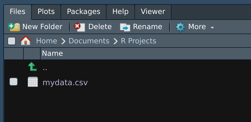
RStudio Files Pane

Where is my data?

Absolute Paths

OS	Path
LINUX	/home/steffi/Documents/R Projects/mydata.csv
WINDOWS	C:/Users/steffi/My Documents/R Projects/mydata.csv
MAC	/users/steffi/Documents/R Projects/mydata.csv

Full location, folders and filename

Relative Paths

Path	Where to look
mydata.csv	Here (current directory)
../mydata.csv	Go up one directory (../)
data/mydata.csv	Stay here, go into “data” folder (data/)
../data/mydata.csv	Go up one directory (../), then into “data” folder (data/)

Only relative info
Use relative symbols (e.g., ../)

With RStudio ‘Projects’ only need to use relative paths

Keep yourself organized

For simple projects

• Create an ‘RStudio Project’ for each Project
• Create a specific “data” folder within each project (one per project)

- Prospect Lake Quality                 # Project Folder
    - prospect_analysis.R
    - data                              # Data Folder   
        - prospect_data_2017-01-01.csv
        - prospect_data_2017-02-01.csv

• Use relative paths to refer to this folder

d <- read_csv("data/prospect_data_2017-01-01.csv")

Let’s Load Some Data!

Your turn: Load some data

1. Create a ‘data’ folder in your RStudio project

2. Put rivers_correct.xlsx file in the “data” folder

3. Load the package

library(readxl)

4. Read in the Excel file and assign to object rivers

rivers <- read_excel("data/rivers_correct.xlsx")

5. Use head() and tail() functions to look at the data
   e.g., head(rivers) and tail(rivers)

6. Click on the rivers object in your “Environment” pane to look at the whole data set

Click on “New Folder”

Use the ‘tab’ key in RStudio when typing in the file name for auto-complete

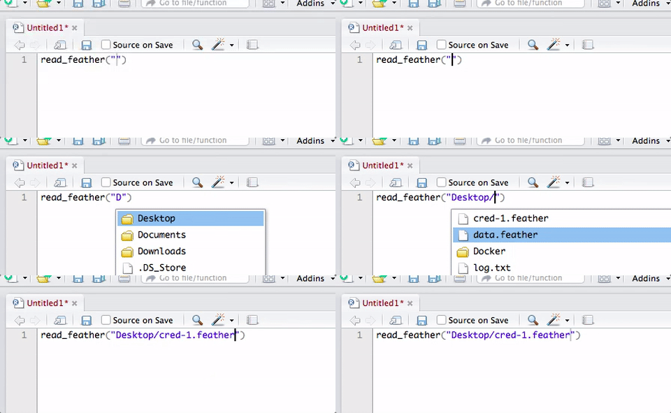
Your turn: Load some data

library(readxl)
rivers <- read_excel("data/rivers_correct.xlsx")

head(rivers)

# A tibble: 6 × 7
  `River Name` Site        Ele      Amo `Temperature C°`  Year Wea   
  <chr>        <chr>       <chr>  <dbl>            <dbl> <dbl> <chr> 
1 Grasse       Up stream   Al    0.606            10.9    2019 cloudy
2 Grasse       Mid stream  Al    0.425             8.68   2020 cloudy
3 Grase        Down stream Al    0.194             8.75   2021 snowy 
4 Oswegatchie  Up stream   Al    1                 0.791  2022 sunny 
5 Oswegatchie  Mid stream  Al    0.161             9.32   2023 cloudy
6 Oswegatchie  Down stream Al    0.0333           10.6    2019 cloudy

tail(rivers)

# A tibble: 6 × 7
  `River Name` Site        Ele      Amo `Temperature C°`  Year Wea   
  <chr>        <chr>       <chr>  <dbl>            <dbl> <dbl> <chr> 
1 Raquette     Up stream   Zr     0.333            14.0   2023 wet   
2 Raquette     Mid stream  Zr     0.111             7.61  2019 wet   
3 Raquette     Down stream Zr    NA                 7.36  2020 wet   
4 St. Regis    Up stream   Zr     0.889             7.94  2021 sunny 
5 St. Regis    Mid stream  Zr     0.778             9.28  2022 snowy 
6 St. Regis    Down stream Zr     0.667            10.1   2023 cloudy

How do I know which function to use?

Program-specific files

• Files which only normally open in a particular program (e.g., Excel)
• Load with function from specific package (e.g. read_excel from readxl package)

Text files

• Files which open in notepad
• Files which open in RStudio when you click on them in the Files Pane
• Load with function from readr package (e.g. read_csv(), read_tsv(), etc.)

Look at the file extension:

• rivers_correct.xlsx Excel file read_excel()
• rivers_raw.csv Comma-separated-variables read_csv()

But sometimes not clear…

How do I know which function to use?

Look at the file: master_moch.txt

• Put this file in your data folder
• In lower right-hand pane, click on Files
  • Click on data folder
  • Click on master_moch.txt
  • Click “View File” (if asked)

ID  region  hab freq    freq.sd p.notes
MCB02   kam 0.5266879074    3.9806600009    3.9806600009    0.4592592593
MCB03   kam -0.9707703735   4.1090031783    4.1090031783    0.5
MCB04   kam -0.9707703735   4.2463067674    4.2463067674    0.5151515152

This does not read the file into R, but only shows you the contents as text.

Hmm, not comma-separated, maybe tab-separated?

How do I know which function to use?

Peak:

• Pick a read function with your best guess (read_csv() is a good start)
• Use n_max to read only first few rows

read_csv("data/master_moch.txt", n_max = 3)

# A tibble: 3 × 1
  `ID\tregion\thab\tfreq\tfreq.sd\tp.notes`                            
  <chr>                                                                
1 "MCB02\tkam\t0.5266879074\t3.9806600009\t3.9806600009\t0.4592592593" 
2 "MCB03\tkam\t-0.9707703735\t4.1090031783\t4.1090031783\t0.5"         
3 "MCB04\tkam\t-0.9707703735\t4.2463067674\t4.2463067674\t0.5151515152"

\t means tab, so this is tab-separated data

How do I know what to use?

Peak:

• Try again with read_tsv()

read_tsv("data/master_moch.txt", n_max = 3)  # note change in function!

# A tibble: 3 × 6
  ID    region    hab  freq freq.sd p.notes
  <chr> <chr>   <dbl> <dbl>   <dbl>   <dbl>
1 MCB02 kam     0.527  3.98    3.98   0.459
2 MCB03 kam    -0.971  4.11    4.11   0.5  
3 MCB04 kam    -0.971  4.25    4.25   0.515

Excellent!

Specifics of loading functions

col_names

• Geolocator data

my_data <- read_csv("data/geolocators.csv")
my_data

# A tibble: 20 × 2
   `02/05/11 22:29:59`  `64`
   <chr>               <dbl>
 1 02/05/11 22:31:59      64
 2 02/05/11 22:33:59      38
 3 02/05/11 22:35:59      38
 4 02/05/11 22:37:59      34
 5 02/05/11 22:39:59      30
 6 02/05/11 22:41:59      34
 7 02/05/11 22:43:59      40
 8 02/05/11 22:45:59      46
 9 02/05/11 22:47:59      48
10 02/05/11 22:49:59      46
# ℹ 10 more rows

Oops?

• read_csv, read_tsv, etc. assume that the first row contains the column names
• This file doesn’t have headers

col_names

• Geolocator data

Declare no headings

my_data <- read_csv("data/geolocators.csv", 
                    col_names = FALSE)
my_data

# A tibble: 21 × 2
   X1                   X2
   <chr>             <dbl>
 1 02/05/11 22:29:59    64
 2 02/05/11 22:31:59    64
 3 02/05/11 22:33:59    38
 4 02/05/11 22:35:59    38
 5 02/05/11 22:37:59    34
 6 02/05/11 22:39:59    30
 7 02/05/11 22:41:59    34
 8 02/05/11 22:43:59    40
 9 02/05/11 22:45:59    46
10 02/05/11 22:47:59    48
# ℹ 11 more rows

Name headings

my_data <- read_csv("data/geolocators.csv", 
                    col_names = c("date", "light"))
my_data

# A tibble: 21 × 2
   date              light
   <chr>             <dbl>
 1 02/05/11 22:29:59    64
 2 02/05/11 22:31:59    64
 3 02/05/11 22:33:59    38
 4 02/05/11 22:35:59    38
 5 02/05/11 22:37:59    34
 6 02/05/11 22:39:59    30
 7 02/05/11 22:41:59    34
 8 02/05/11 22:43:59    40
 9 02/05/11 22:45:59    46
10 02/05/11 22:47:59    48
# ℹ 11 more rows

skip info rows before data

• Grain size data

my_data <- read_tsv("data/grain_size.txt")
my_data

# A tibble: 36 × 7
   `DATA DOWNLOAD: 2015-09-23` ...2  ...3        ...4     ...5  ...6  ...7 
   <chr>                       <chr> <chr>       <chr>    <chr> <chr> <chr>
 1 SYSTEM 001                  <NA>  <NA>        <NA>     <NA>  <NA>  <NA> 
 2 LOGGER X                    <NA>  <NA>        <NA>     <NA>  <NA>  <NA> 
 3 lab_num                     CSP   sample_num  depth_lb csa   msa   fsa  
 4 3177                        CSP01 CSP01-P-1-1 4        13.04 17.37 8.19 
 5 3178                        CSP01 CSP01-P-1-2 12       10.74 16.9  7.92 
 6 3179                        CSP01 CSP01-P-1-3 35       12.11 17.75 6.99 
 7 3180                        CSP01 CSP01-P-1-4 53       17.61 18.16 6.29 
 8 3181                        CSP01 CSP01-P-1-5 83       21.05 18.38 6.26 
 9 3182                        CSP01 CSP01-P-1-6 105      19.02 18.43 6.28 
10 3183                        CSP08 CSP08-P-1-1 10       11.6  17.14 8.18 
# ℹ 26 more rows

skip info rows before data

• Grain size data

my_data <- read_tsv("data/grain_size.txt")
my_data

Look at the file:

• Click on Files tab
• Click on data folder
• Click on grain_size.txt
• Click “View file” (if asked)

DATA DOWNLOAD: 2015-09-23                       
SYSTEM 001                      
LOGGER X                        
lab_num CSP sample_num  depth_lb    csa msa fsa
3177    CSP01   CSP01-P-1-1 4   13.04   17.37   8.19
3178    CSP01   CSP01-P-1-2 12  10.74   16.9    7.92
3179    CSP01   CSP01-P-1-3 35  12.11   17.75   6.99
3180    CSP01   CSP01-P-1-4 53  17.61   18.16   6.29
3181    CSP01   CSP01-P-1-5 83  21.05   18.38   6.26

Ah ha!
Metadata was stored at the top of the file

skip info rows before data

• Grain size data
• Add skip = 3 to skip the first three rows

my_data <- read_tsv("data/grain_size.txt", skip = 3)
my_data

# A tibble: 33 × 7
   lab_num CSP   sample_num  depth_lb   csa   msa   fsa
     <dbl> <chr> <chr>          <dbl> <dbl> <dbl> <dbl>
 1    3177 CSP01 CSP01-P-1-1        4 13.0  17.4   8.19
 2    3178 CSP01 CSP01-P-1-2       12 10.7  16.9   7.92
 3    3179 CSP01 CSP01-P-1-3       35 12.1  17.8   6.99
 4    3180 CSP01 CSP01-P-1-4       53 17.6  18.2   6.29
 5    3181 CSP01 CSP01-P-1-5       83 21.0  18.4   6.26
 6    3182 CSP01 CSP01-P-1-6      105 19.0  18.4   6.28
 7    3183 CSP08 CSP08-P-1-1       10 11.6  17.1   8.18
 8    3184 CSP08 CSP08-P-1-2       27 15.4  16.2   6.76
 9    3185 CSP08 CSP08-P-1-3       90 14.9  15.8   7.12
10    3186 CSP02 CSP02-P-1-1        5  8.75  8.64  3.41
# ℹ 23 more rows

Much better!

Your turn: Load this data set

Load the telemetry data set: Sta A Data 2006-11-07.dmp

1. Look at the file
2. Decide which R function to use based on delimiter (comma, space, or tab?)
3. Any other options need to be specified?

It should look like this:

# A tibble: 19 × 7
  StartDate Time     Frequency `Rate/Temp`   Pwr Ant      SD
      <dbl> <time>       <dbl>       <dbl> <dbl> <chr> <dbl>
1     39022 17:15:36      150.        34.8   175 M0        0
2     39022 17:19:14      148.        19.2    72 M0        0
3     39022 17:19:25      148.        19.7   194 M1        0
4     39022 17:20:04      149.        33.8   104 M0        0
5     39022 17:20:17      149.        33.7   152 M1        0
6     39022 17:20:57      150.        34.2   188 M0        0
7     39022 17:22:50      148.         9.8   188 M0        0
# ℹ 12 more rows

Too Easy?
Load some of your own tricky data OR
Try to load the second sheet of rivers_correct.xlsx and rename the columns in the same step
(see ?read_excel)

Your turn: Load this data set

Load the telemetry data set: Sta A Data 2006-11-07.dmp

telemetry <- read_csv("data/Sta A Data 2006-11-07.dmp", skip = 2)
telemetry

# A tibble: 19 × 7
  StartDate Time     Frequency `Rate/Temp`   Pwr Ant      SD
      <dbl> <time>       <dbl>       <dbl> <dbl> <chr> <dbl>
1     39022 17:15:36      150.        34.8   175 M0        0
2     39022 17:19:14      148.        19.2    72 M0        0
3     39022 17:19:25      148.        19.7   194 M1        0
4     39022 17:20:04      149.        33.8   104 M0        0
5     39022 17:20:17      149.        33.7   152 M1        0
6     39022 17:20:57      150.        34.2   188 M0        0
7     39022 17:22:50      148.         9.8   188 M0        0
# ℹ 12 more rows

Your turn: Load this data set

Too Easy?

• Use sheet argument to access specific sheet (excel_sheets() lists them all)
• skip the first three rows (including the headers)
• provide new header names

excel_sheets("data/rivers_correct.xlsx")  # Or look yourself ;)

[1] "Sheet1"      "Oswegatchie"

read_excel("data/rivers_correct.xlsx", sheet = "Oswegatchie", skip = 3, 
           col_names = c("name", "site", "element", "amount", 
                         "temp", "year", "weather"))

# A tibble: 75 × 7
   name        site        element  amount   temp  year weather
   <chr>       <chr>       <chr>     <dbl>  <dbl> <dbl> <chr>  
 1 Oswegatchie Up stream   Al       1       0.791  2022 sunny  
 2 Oswegatchie Mid stream  Al       0.161   9.32   2023 cloudy 
 3 Oswegatchie Down stream Al       0.0333 10.6    2019 cloudy 
 4 Oswegatchie Up stream   Ba       0.357   3.73   2019 cloudy 
 5 Oswegatchie Mid stream  Ba       0.560   9.66   2020 sunny  
 6 Oswegatchie Down stream Ba       1       8.56   2021 wet    
 7 Oswegatchie Up stream   Br       0.107  20.9    2021 sunny  
 8 Oswegatchie Mid stream  Br       0.857  10.8    2022 sunny  
 9 Oswegatchie Down stream Br       1       4.79   2023 cloudy 
10 Oswegatchie Up stream   Ca      NA       4.76   2023 cloudy 
# ℹ 65 more rows

Looking for problems

Look at the data

• Make sure columns as expected (correctly assigned file format)
• Make sure no extra lines above the data (should we have used a skip?)
• Make sure column names look appropriate

library(palmerpenguins)
penguins

# A tibble: 344 × 8
   species island    bill_length_mm bill_depth_mm flipper_length_mm body_mass_g sex     year
   <fct>   <fct>              <dbl>         <dbl>             <int>       <int> <fct>  <int>
 1 Adelie  Torgersen           39.1          18.7               181        3750 male    2007
 2 Adelie  Torgersen           39.5          17.4               186        3800 female  2007
 3 Adelie  Torgersen           40.3          18                 195        3250 female  2007
 4 Adelie  Torgersen           NA            NA                  NA          NA <NA>    2007
 5 Adelie  Torgersen           36.7          19.3               193        3450 female  2007
 6 Adelie  Torgersen           39.3          20.6               190        3650 male    2007
 7 Adelie  Torgersen           38.9          17.8               181        3625 female  2007
 8 Adelie  Torgersen           39.2          19.6               195        4675 male    2007
 9 Adelie  Torgersen           34.1          18.1               193        3475 <NA>    2007
10 Adelie  Torgersen           42            20.2               190        4250 <NA>    2007
# ℹ 334 more rows

Look at the data

• Did the whole data set load?
• Are there extra blank lines at the end of the data?

tail(penguins)

# A tibble: 6 × 8
  species   island bill_length_mm bill_depth_mm flipper_length_mm body_mass_g sex     year
  <fct>     <fct>           <dbl>         <dbl>             <int>       <int> <fct>  <int>
1 Chinstrap Dream            45.7          17                 195        3650 female  2009
2 Chinstrap Dream            55.8          19.8               207        4000 male    2009
3 Chinstrap Dream            43.5          18.1               202        3400 female  2009
4 Chinstrap Dream            49.6          18.2               193        3775 male    2009
5 Chinstrap Dream            50.8          19                 210        4100 male    2009
6 Chinstrap Dream            50.2          18.7               198        3775 female  2009

skim() the data

skim() is from skimr

• Are the formats correct?
  • numbers (numeric),
  • text (character)
  • date (date, POSIXct, datetime)
  • categories (factor)
• Are values appropriate?
  • Should there be NAs?
• Are there any typos?
• Number of rows expected?

library(skimr)
skim(penguins)

── Data Summary ────────────────────────
                           Values  
Name                       penguins
Number of rows             344     
Number of columns          8       
_______________________            
Column type frequency:             
  factor                   3       
  numeric                  5       
________________________           
Group variables            None    

── Variable type: factor ───────────────────────────────────────────────────────────────────────────────────────────────────────────────────────────────────────────────────────────────────────────────
  skim_variable n_missing complete_rate ordered n_unique top_counts                 
1 species               0         1     FALSE          3 Ade: 152, Gen: 124, Chi: 68
2 island                0         1     FALSE          3 Bis: 168, Dre: 124, Tor: 52
3 sex                  11         0.968 FALSE          2 mal: 168, fem: 165         

── Variable type: numeric ──────────────────────────────────────────────────────────────────────────────────────────────────────────────────────────────────────────────────────────────────────────────
  skim_variable     n_missing complete_rate   mean      sd     p0    p25    p50    p75   p100 hist 
1 bill_length_mm            2         0.994   43.9   5.46    32.1   39.2   44.4   48.5   59.6 ▃▇▇▆▁
2 bill_depth_mm             2         0.994   17.2   1.97    13.1   15.6   17.3   18.7   21.5 ▅▅▇▇▂
3 flipper_length_mm         2         0.994  201.   14.1    172    190    197    213    231   ▂▇▃▅▂
4 body_mass_g               2         0.994 4202.  802.    2700   3550   4050   4750   6300   ▃▇▆▃▂
5 year                      0         1     2008.    0.818 2007   2007   2008   2009   2009   ▇▁▇▁▇

count() categories

count() is from dplyr*

• Check for sample sizes and potential typos in categorical columns
• Assess missing values

count(penguins, species)

# A tibble: 3 × 2
  species       n
  <fct>     <int>
1 Adelie      152
2 Chinstrap    68
3 Gentoo      124

count(penguins, island)

# A tibble: 3 × 2
  island        n
  <fct>     <int>
1 Biscoe      168
2 Dream       124
3 Torgersen    52

count(penguins, sex)

# A tibble: 3 × 2
  sex        n
  <fct>  <int>
1 female   165
2 male     168
3 <NA>      11

* part of the tidyverse

Plot categories

# Replace COLUMN with the column name to explore
ggplot(data = penguins, aes(x = COLUMN)) + 
  geom_bar()

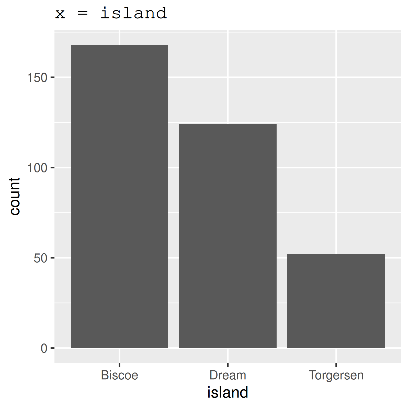
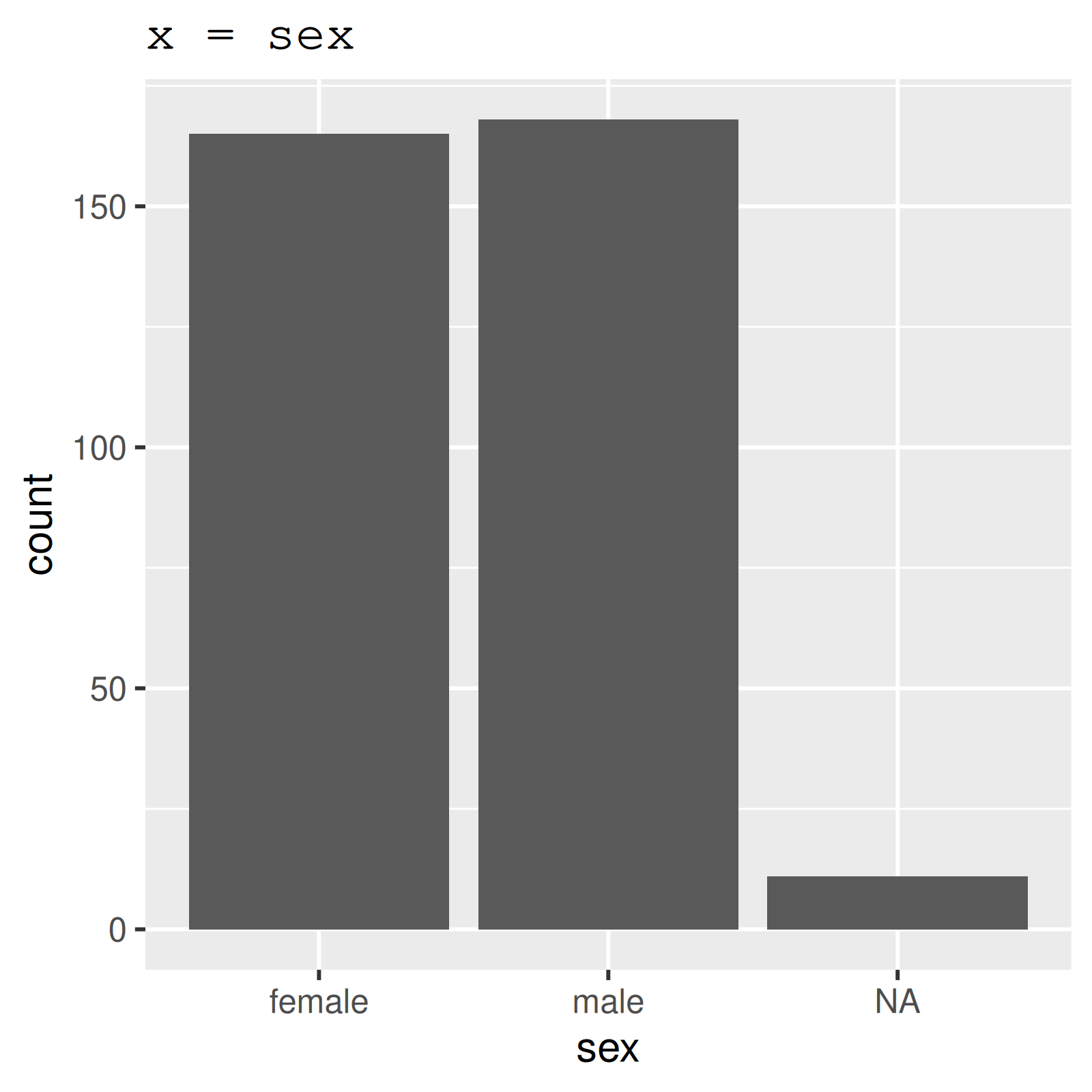
* part of the tidyverse

Plot numbers

# Replace COLUMN with the column name to explore
ggplot(data = penguins, aes(x = COLUMN)) + 
  geom_histogram()

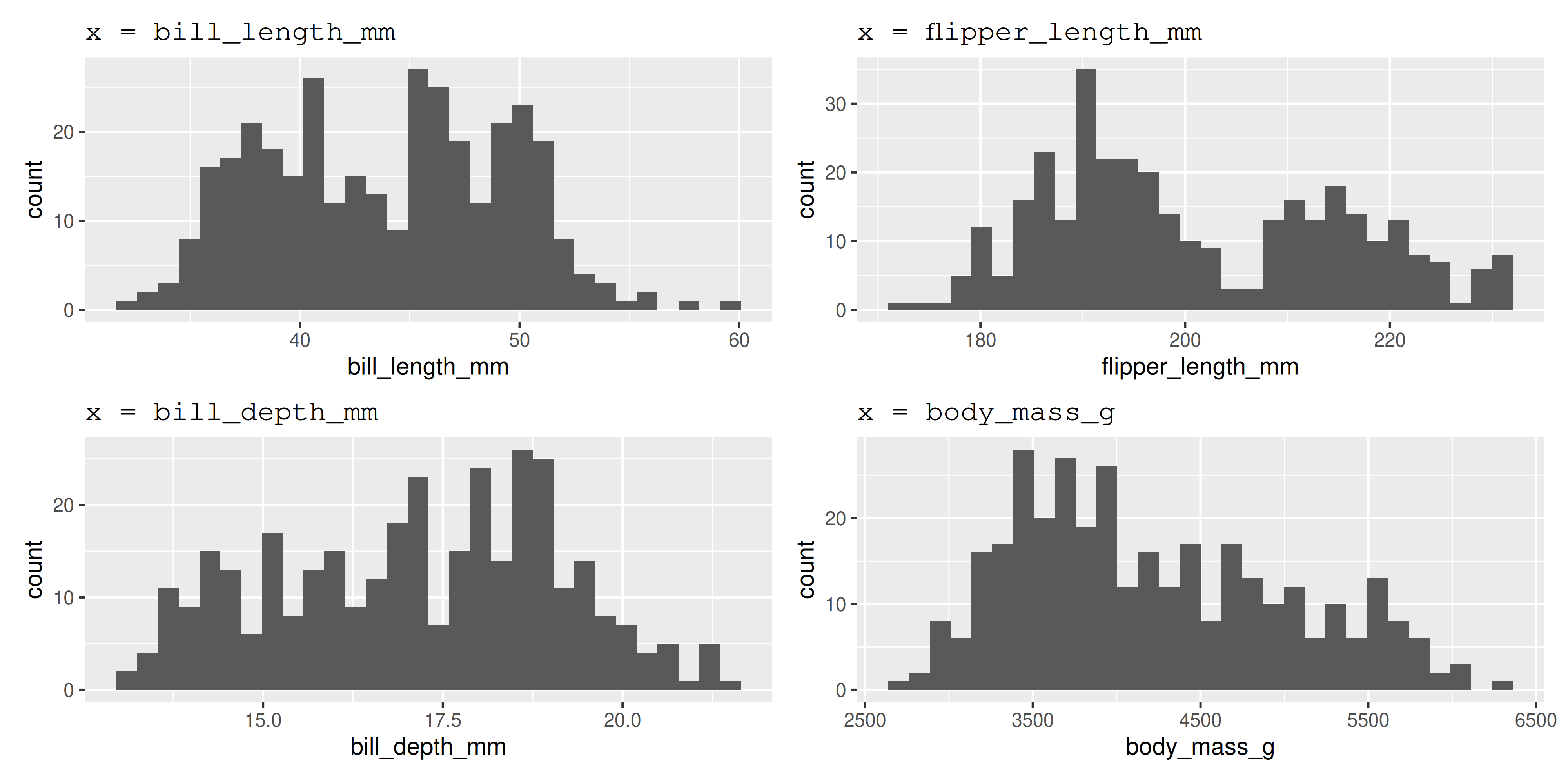
* part of the tidyverse

Example of problematic data

rivers_raw.csv

Look at the data

rivers <- read_csv("data/rivers_raw.csv")
rivers

# A tibble: 300 × 7
   `River Name` Site        Ele       Amo `Temperature C°`  Year Wea   
   <chr>        <chr>       <chr>   <dbl>            <dbl> <dbl> <chr> 
 1 Grasse       Up stream   Al     0.606            10.9    2019 sunny 
 2 Grasse       Mid stream  Al     0.425             8.68   2020 sunny 
 3 Grase        Down stream Al     0.194             8.75   2021 sunny 
 4 Oswegatchie  Up stream   Al     1                 0.791  2022 snowy 
 5 Oswegatchie  Mid stream  Al     0.161             9.32   2023 sunny 
 6 Oswegatchie  Down stream Al     0.0333           10.6    2019 wet   
 7 Raquette     Up stream   Al     0.292             4.01   2020 cloudy
 8 Raquette     Mid stream  Al     0.0389            5.96   2021 wet   
 9 Raquette     Down stream Al    NA                 6.21   2022 wet   
10 St. Regis    Up stream   Al     0.681             8.02   2023 cloudy
# ℹ 290 more rows

• Column names are not R-friendly (River Name and Temperature C°) or obvious (what is Ele?)
• At least one typo in River (Grase should be Grasse)

Looking for problems

Your Turn!

rivers <- read_csv("data/rivers_raw.csv")
rivers

# A tibble: 300 × 7
   `River Name` Site        Ele       Amo `Temperature C°`  Year Wea   
   <chr>        <chr>       <chr>   <dbl>            <dbl> <dbl> <chr> 
 1 Grasse       Up stream   Al     0.606            10.9    2019 sunny 
 2 Grasse       Mid stream  Al     0.425             8.68   2020 sunny 
 3 Grase        Down stream Al     0.194             8.75   2021 sunny 
 4 Oswegatchie  Up stream   Al     1                 0.791  2022 snowy 
 5 Oswegatchie  Mid stream  Al     0.161             9.32   2023 sunny 
 6 Oswegatchie  Down stream Al     0.0333           10.6    2019 wet   
 7 Raquette     Up stream   Al     0.292             4.01   2020 cloudy
 8 Raquette     Mid stream  Al     0.0389            5.96   2021 wet   
 9 Raquette     Down stream Al    NA                 6.21   2022 wet   
10 St. Regis    Up stream   Al     0.681             8.02   2023 cloudy
# ℹ 290 more rows

• skim() the data
• count() some columns
• Perhaps make some ggplot()s

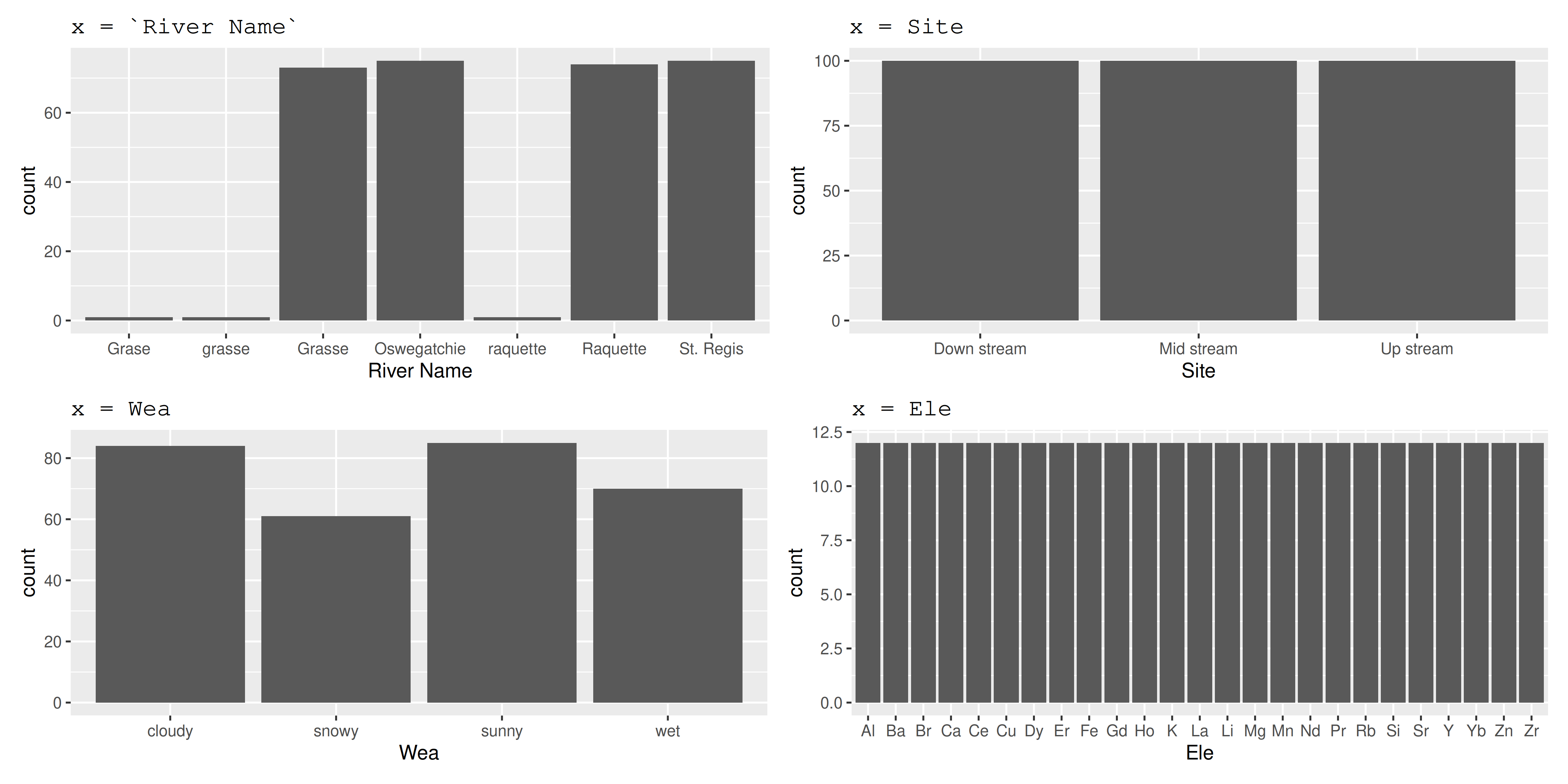
Find any problems?

skim() the data

skim(rivers)

── Data Summary ────────────────────────
                           Values
Name                       rivers
Number of rows             300   
Number of columns          7     
_______________________          
Column type frequency:           
  character                4     
  numeric                  3     
________________________         
Group variables            None  

── Variable type: character ──────────────────────────────────────────────────────────────────────────────────
  skim_variable n_missing complete_rate min max empty n_unique whitespace
1 River Name            0             1   5  11     0        7          0
2 Site                  0             1   9  11     0        3          0
3 Ele                   0             1   1   2     0       25          0
4 Wea                   0             1   3   6     0        4          0

── Variable type: numeric ────────────────────────────────────────────────────────────────────────────────────
  skim_variable  n_missing complete_rate     mean     sd         p0      p25      p50      p75   p100 hist 
1 Amo                   39          0.87    0.429  0.299    0.00656    0.169    0.379    0.643    1   ▇▆▆▃▃
2 Temperature C°         0          1       9.17  11.5    -99          7.54    10.3     12.7     20.9 ▁▁▁▁▇
3 Year                   0          1    2021      1.42  2019       2020     2021     2022     2023   ▇▇▇▇▇

count() categories

count(rivers, `River Name`)

# A tibble: 7 × 2
  `River Name`     n
  <chr>        <int>
1 Grase            1
2 Grasse          73
3 Oswegatchie     75
4 Raquette        74
5 St. Regis       75
6 grasse           1
7 raquette         1

count(rivers, Wea)

# A tibble: 4 × 2
  Wea        n
  <chr>  <int>
1 cloudy    85
2 snowy     66
3 sunny     72
4 wet       77

count(rivers, Site)

# A tibble: 3 × 2
  Site            n
  <chr>       <int>
1 Down stream   100
2 Mid stream    100
3 Up stream     100

count(rivers, Ele)

# A tibble: 25 × 2
   Ele       n
   <chr> <int>
 1 Al       12
 2 Ba       12
 3 Br       12
 4 Ca       12
 5 Ce       12
 6 Cu       12
 7 Dy       12
 8 Er       12
 9 Fe       12
10 Gd       12
# ℹ 15 more rows

Plot categories

# Replace COLUMN with the column name to explore
ggplot(data = rivers, aes(x = COLUMN)) + 
  geom_bar()

Plot numbers

# Replace COLUMN with the column name to explore
ggplot(data = rivers, aes(x = COLUMN)) + 
  geom_histogram()()

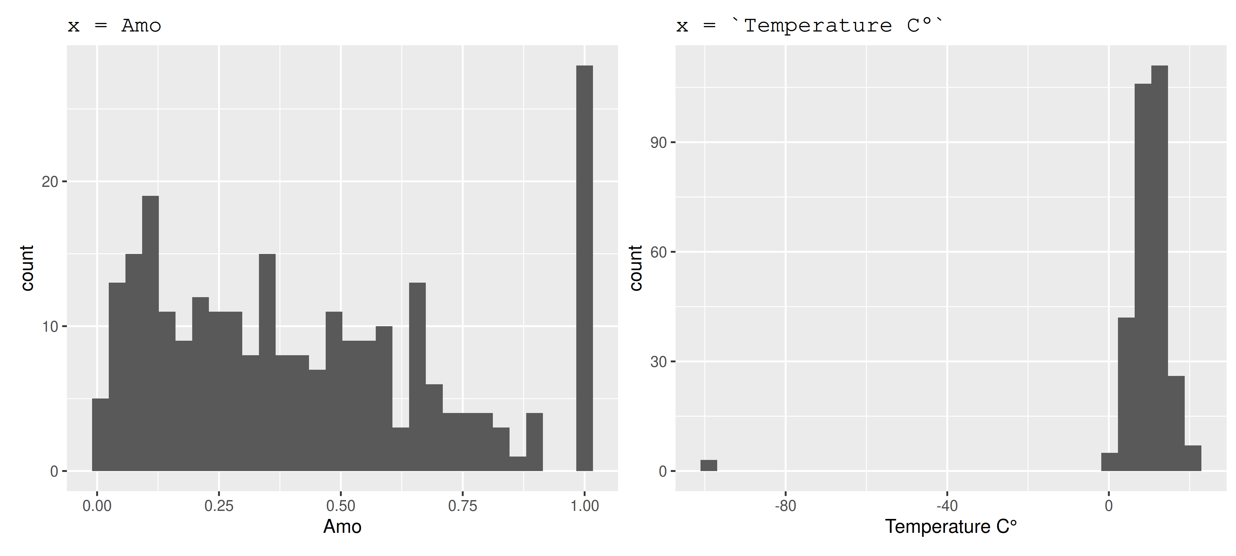
Fixing problems

Cleaning column names

clean_names() is from janitor*

* not part of the tidyverse but tidyverse-orientated

library(janitor)
rivers <- clean_names(rivers)
rivers

# A tibble: 300 × 7
   river_name  site        ele       amo temperature_c  year wea   
   <chr>       <chr>       <chr>   <dbl>         <dbl> <dbl> <chr> 
 1 Grasse      Up stream   Al     0.606         10.9    2019 sunny 
 2 Grasse      Mid stream  Al     0.425          8.68   2020 sunny 
 3 Grase       Down stream Al     0.194          8.75   2021 sunny 
 4 Oswegatchie Up stream   Al     1              0.791  2022 snowy 
 5 Oswegatchie Mid stream  Al     0.161          9.32   2023 sunny 
 6 Oswegatchie Down stream Al     0.0333        10.6    2019 wet   
 7 Raquette    Up stream   Al     0.292          4.01   2020 cloudy
 8 Raquette    Mid stream  Al     0.0389         5.96   2021 wet   
 9 Raquette    Down stream Al    NA              6.21   2022 wet   
10 St. Regis   Up stream   Al     0.681          8.02   2023 cloudy
# ℹ 290 more rows

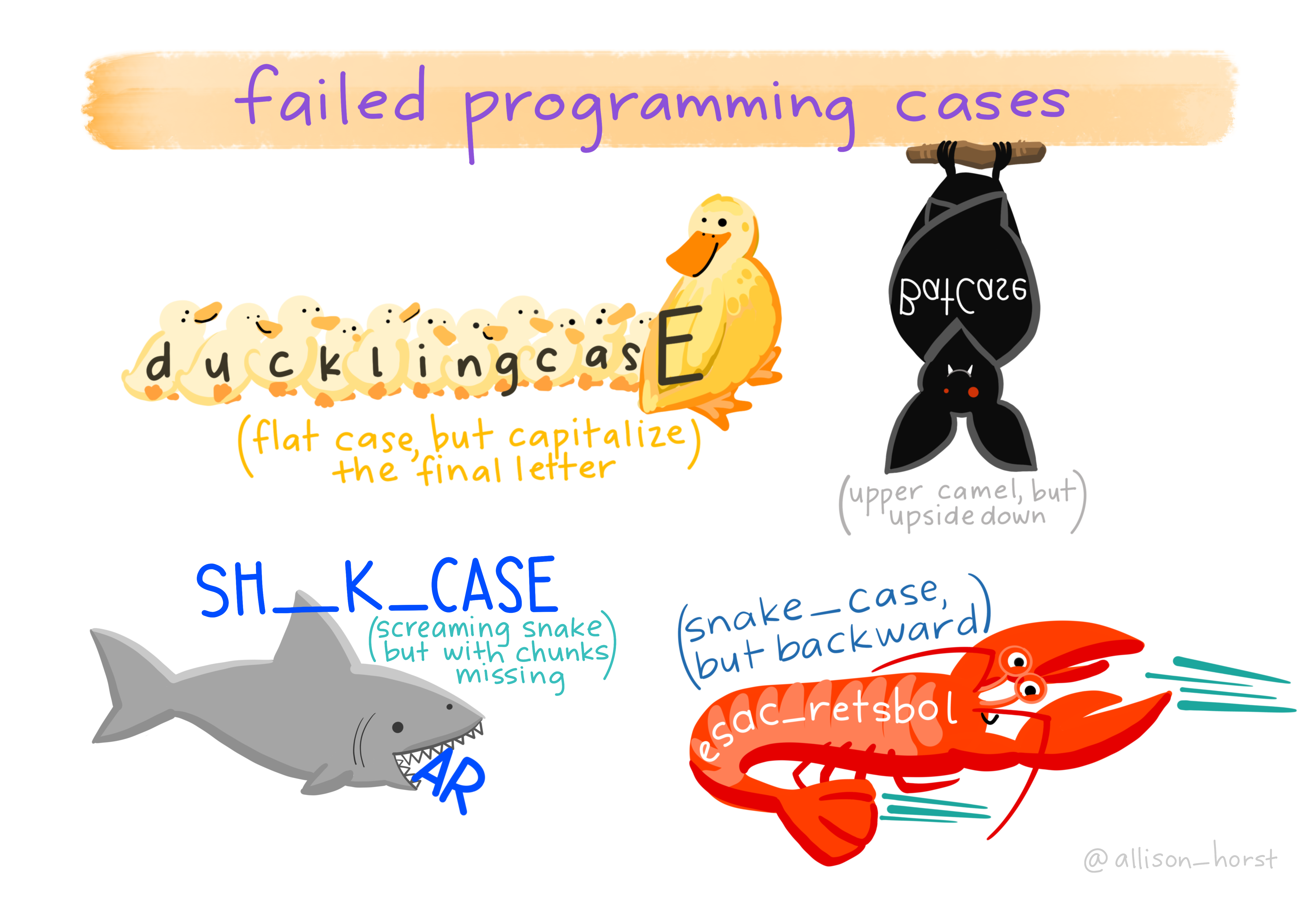
Side Note: Naming conventions

Side Note: Naming conventions

Cleaning column names

rename() is from dplyr*

rename() columns

rivers <- rename(rivers, element = ele, amount = amo, temperature = temperature_c)
rivers

# A tibble: 300 × 7
   river_name  site        element  amount temperature  year wea   
   <chr>       <chr>       <chr>     <dbl>       <dbl> <dbl> <chr> 
 1 Grasse      Up stream   Al       0.606       10.9    2019 sunny 
 2 Grasse      Mid stream  Al       0.425        8.68   2020 sunny 
 3 Grase       Down stream Al       0.194        8.75   2021 sunny 
 4 Oswegatchie Up stream   Al       1            0.791  2022 snowy 
 5 Oswegatchie Mid stream  Al       0.161        9.32   2023 sunny 
 6 Oswegatchie Down stream Al       0.0333      10.6    2019 wet   
 7 Raquette    Up stream   Al       0.292        4.01   2020 cloudy
 8 Raquette    Mid stream  Al       0.0389       5.96   2021 wet   
 9 Raquette    Down stream Al      NA            6.21   2022 wet   
10 St. Regis   Up stream   Al       0.681        8.02   2023 cloudy
# ℹ 290 more rows

* part of the tidyverse

Subsetting columns

select() is from dplyr*

select() columns you want

rivers <- select(rivers, river_name, site, element, amount)

* part of the tidyverse

OR, unselect() columns you don’t want

rivers <- select(rivers, -wea)
rivers

# A tibble: 300 × 6
   river_name  site        element  amount temperature  year
   <chr>       <chr>       <chr>     <dbl>       <dbl> <dbl>
 1 Grasse      Up stream   Al       0.606       10.9    2019
 2 Grasse      Mid stream  Al       0.425        8.68   2020
 3 Grase       Down stream Al       0.194        8.75   2021
 4 Oswegatchie Up stream   Al       1            0.791  2022
 5 Oswegatchie Mid stream  Al       0.161        9.32   2023
 6 Oswegatchie Down stream Al       0.0333      10.6    2019
 7 Raquette    Up stream   Al       0.292        4.01   2020
 8 Raquette    Mid stream  Al       0.0389       5.96   2021
 9 Raquette    Down stream Al      NA            6.21   2022
10 St. Regis   Up stream   Al       0.681        8.02   2023
# ℹ 290 more rows

Cleaning columns

Put it all together

rivers <- read_csv("data/rivers_raw.csv")
rivers <- clean_names(rivers)
rivers <- rename(rivers, element = ele, amount = amo, temperature = temperature_c)
rivers <- select(rivers, -wea)
rivers

# A tibble: 300 × 6
   river_name  site        element  amount temperature  year
   <chr>       <chr>       <chr>     <dbl>       <dbl> <dbl>
 1 Grasse      Up stream   Al       0.606       10.9    2019
 2 Grasse      Mid stream  Al       0.425        8.68   2020
 3 Grase       Down stream Al       0.194        8.75   2021
 4 Oswegatchie Up stream   Al       1            0.791  2022
 5 Oswegatchie Mid stream  Al       0.161        9.32   2023
 6 Oswegatchie Down stream Al       0.0333      10.6    2019
 7 Raquette    Up stream   Al       0.292        4.01   2020
 8 Raquette    Mid stream  Al       0.0389       5.96   2021
 9 Raquette    Down stream Al      NA            6.21   2022
10 St. Regis   Up stream   Al       0.681        8.02   2023
# ℹ 290 more rows

Note how code repeats data frame rivers…

Fixing typos

Remember the typos…

count(rivers, river_name)

# A tibble: 7 × 2
  river_name      n
  <chr>       <int>
1 Grase           1
2 Grasse         73
3 Oswegatchie    75
4 Raquette       74
5 St. Regis      75
6 grasse          1
7 raquette        1

Fixing typos

Replace typos

Combine the if_else function with the mutate() function

rivers <- mutate(rivers, river_name = if_else(river_name == "Grase", "Grasse", river_name))

Check that it’s gone:

count(rivers, river_name)

# A tibble: 6 × 2
  river_name      n
  <chr>       <int>
1 Grasse         74
2 Oswegatchie    75
3 Raquette       74
4 St. Regis      75
5 grasse          1
6 raquette        1

Fixing typos

if_else() and mutate() from dplyr package*

mutate() creates or changes columns in a data frame:

mutate(dataframe, column = new_values)

if_else() tests for a condition, and returns one value if FALSE and another if TRUE

if_else(condition, value_if_true, value_if_false)

* part of the tidyverse

Iterative process

• Make some corrections
• Check the data
• Make some more corrections (either add to or modify existing code)

Many corrections?

Try case_when() from dplyr package*

case_when() tests for multiple conditions, and returns different values depending

case_when(condition1 ~ value_if_true1,
          condition2 ~ value_if_true2,
          condition3 ~ value_if_true3,
          TRUE ~ default_value)

* part of the tidyverse

Your Turn: Fix another “Grasse” typo

1. Check the data with count()
2. Use mutate() and if_else() to fix the typo

rivers <- read_csv("data/rivers_raw.csv")
rivers <- clean_names(rivers)
rivers <- rename(rivers, element = ele, amount = amo, temperature = temperature_c)
rivers <- select(rivers, -wea)
rivers <- mutate(rivers, river_name = if_else(river_name == "Grase", "Grasse", river_name))

rivers <- mutate(???, ??? = ???)

Too Easy?
Examine and fix problems in your own data OR
Use case_when() to fix all the river name typos at once…

Your Turn: Fix another “Grasse” typo

1. Check the data with count()
2. Use mutate() and if_else() to fix the typo

rivers <- read_csv("data/rivers_raw.csv")
rivers <- clean_names(rivers)
rivers <- rename(rivers, element = ele, amount = amo, temperature = temperature_c)
rivers <- select(rivers, -wea)
rivers <- mutate(rivers, river_name = if_else(river_name == "Grase", "Grasse", river_name))

rivers <- mutate(rivers, river_name = if_else(river_name == "grasse", "Grasse", river_name))

Fixing typos

To be more efficient, fix all typos at once

rivers <- read_csv("data/rivers_raw.csv")
rivers <- clean_names(rivers)
rivers <- rename(rivers, element = ele, amount = amo, temperature = temperature_c)
rivers <- select(rivers, -wea)
rivers <- mutate(rivers, 
                 river_name = if_else(river_name %in% c("Grase", "grasse"), "Grasse", river_name))

== compares one item to one other
%in% compares one item to many different ones

Fixing typos

One last typo to fix

rivers <- read_csv("data/rivers_raw.csv")
rivers <- clean_names(rivers)
rivers <- rename(rivers, element = ele, amount = amo, temperature = temperature_c)
rivers <- select(rivers, -wea)
rivers <- mutate(rivers, 
                 river_name = if_else(river_name %in% c("Grase","grasse"), "Grasse", river_name),
                 river_name = if_else(river_name == "raquette", "Raquette", river_name))

Combine with case_when()

rivers <- read_csv("data/rivers_raw.csv")
rivers <- clean_names(rivers)
rivers <- rename(rivers, element = ele, amount = amo, temperature = temperature_c)
rivers <- select(rivers, -wea)
rivers <- mutate(rivers, 
                 river_name = case_when(river_name %in% c("Grase", "grasse") ~ "Grasse",
                                        river_name == "raquette" ~ "Raquette",
                                        TRUE ~ river_name))

Tangent: tidyverse functions

tidyverse functions

rename(), select(), mutate()

• tidyverse functions always start with the data, followed by other arguments
• you can reference any column from ‘data’

rivers <- read_csv("data/rivers_raw.csv")
rivers <- clean_names(rivers)
rivers <- rename(rivers, element = ele, amount = amo, temperature = temperature_c)
rivers <- select(rivers, -wea)
rivers <- mutate(rivers, river_name = if_else(river_name %in% c("Grase", "grasse"), "Grasse",  river_name))

• rename() changes column names
• select() chooses columns to keep or to remove (with -)
• mutate() changes column contents

Why use tidyverse functions?

Pipes! |>* Allow you to string commands together

Instead of:

rivers <- read_csv("data/rivers_raw.csv")
rivers <- clean_names(rivers)
rivers <- rename(rivers, element = ele, amount = amo, temperature = temperature_c)
rivers <- select(rivers, -wea)
rivers <- mutate(rivers, 
                 river_name = case_when(river_name %in% c("Grase", "grasse") ~ "Grasse",
                                        river_name == "raquette" ~ "Raquette",
                                        TRUE ~ river_name))

* |> is the base pipe, %>% is the tidyverse pipe, you can use either

We have:

rivers <- read_csv("data/rivers_raw.csv") |>
  clean_names() |>
  rename(element = ele, amount = amo, temperature = temperature_c) |>
  select(-wea) |>
  mutate(river_name = case_when(river_name %in% c("Grase", "grasse") ~ "Grasse",
                                river_name == "raquette" ~ "Raquette",
                                TRUE ~ river_name))

Play around

Take a moment to play with this code in your console

Convert this:

rivers <- read_csv("data/rivers_raw.csv")
rivers <- clean_names(rivers)
rivers <- rename(rivers, element = ele, amount = amo, temperature = temperature_c)
rivers <- select(rivers, -wea)
rivers <- mutate(rivers, 
                 river_name = case_when(river_name %in% c("Grase", "grasse") ~ "Grasse",
                                        river_name == "raquette" ~ "Raquette",
                                        TRUE ~ river_name))

To this:

rivers <- read_csv("data/rivers_raw.csv") |>
  clean_names() |>
  rename(element = ele, amount = amo, temperature = temperature_c) |>
  select(-wea) |>
  mutate(river_name = case_when(river_name %in% c("Grase", "grasse") ~ "Grasse",
                                river_name == "raquette" ~ "Raquette",
                                TRUE ~ river_name))

Dealing with NAs

Data that is missing
Data that should be missing

Exploring NAs

• We saw missing values in amount
• Use filter() to take a closer look

filter(rivers, is.na(amount))

# A tibble: 39 × 6
   river_name  site        element amount temperature  year
   <chr>       <chr>       <chr>    <dbl>       <dbl> <dbl>
 1 Raquette    Down stream Al          NA        6.21  2022
 2 Raquette    Up stream   Ba          NA        5.23  2022
 3 Raquette    Up stream   Br          NA      -99     2019
 4 Oswegatchie Up stream   Ca          NA        4.76  2023
 5 Raquette    Down stream Ce          NA       13.9   2020
 6 Grasse      Up stream   Cu          NA        9.13  2019
 7 Raquette    Down stream Dy          NA        4.98  2019
 8 Raquette    Down stream Er          NA        3.07  2021
 9 Raquette    Down stream Fe          NA        7.20  2023
10 Raquette    Down stream Gd          NA        4.73  2020
# ℹ 29 more rows

Omitting NAs

drop_na() is from tidyr*

Omit NAs from the amount column only (drop those rows)

rivers_no_na <- drop_na(rivers, amount)

Omit all NAs from all columns (drop those rows)

rivers_no_na <- drop_na(rivers)

Check…

filter(rivers_no_na, is.na(amount))

# A tibble: 0 × 6
# ℹ 6 variables: river_name <chr>, site <chr>, element <chr>, amount <dbl>, temperature <dbl>, year <dbl>

nrow(rivers_no_na)

[1] 261

No more NAs!
Fewer rows

* part of the tidyverse

Side Note: filter() also omits NAs 😱

If we filter by the column with NAs, they are silently dropped

filter(rivers, amount < 0.05)

# A tibble: 15 × 6
   river_name  site        element  amount temperature  year
   <chr>       <chr>       <chr>     <dbl>       <dbl> <dbl>
 1 Oswegatchie Down stream Al      0.0333       10.6    2019
 2 Raquette    Mid stream  Al      0.0389        5.96   2021
 3 Grasse      Mid stream  Br      0.0357       12.4    2019
 4 St. Regis   Up stream   Br      0.0357        3.52   2022
 5 St. Regis   Mid stream  Br      0.0357        0.936  2023
 6 Raquette    Mid stream  Ce      0.0116        6.61   2019
 7 Raquette    Mid stream  Fe      0.00656      10.8    2022
 8 Grasse      Up stream   K       0.0313        3.61   2021
 9 Raquette    Mid stream  La      0.0275        2.50   2020
10 Oswegatchie Down stream Mn      0.00672       8.89   2019
# ℹ 5 more rows

We need to be explicit if we want to keep them

filter(rivers, amount < 0.05 | is.na(amount))

# A tibble: 54 × 6
   river_name  site        element  amount temperature  year
   <chr>       <chr>       <chr>     <dbl>       <dbl> <dbl>
 1 Oswegatchie Down stream Al       0.0333      10.6    2019
 2 Raquette    Mid stream  Al       0.0389       5.96   2021
 3 Raquette    Down stream Al      NA            6.21   2022
 4 Raquette    Up stream   Ba      NA            5.23   2022
 5 Grasse      Mid stream  Br       0.0357      12.4    2019
 6 Raquette    Up stream   Br      NA          -99      2019
 7 St. Regis   Up stream   Br       0.0357       3.52   2022
 8 St. Regis   Mid stream  Br       0.0357       0.936  2023
 9 Oswegatchie Up stream   Ca      NA            4.76   2023
10 Raquette    Mid stream  Ce       0.0116       6.61   2019
# ℹ 44 more rows

Replacing NAs

replace_na() is from tidyr*

rivers_no_na <- mutate(rivers, amount = replace_na(amount, 0))

Check…

filter(rivers_no_na, is.na(amount))

# A tibble: 0 × 6
# ℹ 6 variables: river_name <chr>, site <chr>, element <chr>, amount <dbl>, temperature <dbl>, year <dbl>

nrow(rivers_no_na)

[1] 300

No more NAs!
Same number of rows

(If you want to do a more complex replacement, you’ll have to use if_else() or case_when() like we did for typos.)

* part of the tidyverse

Converting to NA

Remember the problem with temperature?

filter(rivers, temperature < -10)

# A tibble: 3 × 6
  river_name  site       element amount temperature  year
  <chr>       <chr>      <chr>    <dbl>       <dbl> <dbl>
1 Raquette    Up stream  Br      NA             -99  2019
2 Oswegatchie Mid stream K        0.426         -99  2020
3 St. Regis   Mid stream La       0.367         -99  2023

na_if() is from dplyr*

rivers <- mutate(rivers, temperature = na_if(temperature, -99))

* part of the tidyverse

Check…

filter(rivers, is.na(temperature))

# A tibble: 3 × 6
  river_name  site       element amount temperature  year
  <chr>       <chr>      <chr>    <dbl>       <dbl> <dbl>
1 Raquette    Up stream  Br      NA              NA  2019
2 Oswegatchie Mid stream K        0.426          NA  2020
3 St. Regis   Mid stream La       0.367          NA  2023

Fixing formats

Changing classes

Function	Input	Output
as.character()	Any vector	Text (Characters)
as.numeric()	Any vector (but returns NAs if not numbers)	Numbers
as.logical()	TRUE, FALSE, T, F, 0 (FALSE), any other number (all TRUE)	TRUE or FALSE
as.factor()	Any vector	Categories

We’ll deal with dates and times later…

Your turn, try the following…

a <- c("hi", "hello", "bonjour")

as.character(a)
as.numeric(a)
as.logical(a)
as.factor(a)

b <- c(1, 0, 20)

as.character(b)
as.numeric(b)
as.logical(b)
as.factor(b)

Changing classes

Your turn, try the following…

a <- c("hi", "hello", "bonjour")

as.character(a)

[1] "hi"      "hello"   "bonjour"

as.numeric(a)

[1] NA NA NA

as.logical(a)

[1] NA NA NA

as.factor(a)

[1] hi      hello   bonjour
Levels: bonjour hello hi

b <- c(1, 0, 20)

as.character(b)

[1] "1"  "0"  "20"

as.numeric(b)

[1]  1  0 20

as.logical(b)

[1]  TRUE FALSE  TRUE

as.factor(b)

[1] 1  0  20
Levels: 0 1 20

Look for problems

rivers

# A tibble: 300 × 6
   river_name  site        element  amount temperature  year
   <chr>       <chr>       <chr>     <dbl>       <dbl> <dbl>
 1 Grasse      Up stream   Al       0.606       10.9    2019
 2 Grasse      Mid stream  Al       0.425        8.68   2020
 3 Grasse      Down stream Al       0.194        8.75   2021
 4 Oswegatchie Up stream   Al       1            0.791  2022
 5 Oswegatchie Mid stream  Al       0.161        9.32   2023
 6 Oswegatchie Down stream Al       0.0333      10.6    2019
 7 Raquette    Up stream   Al       0.292        4.01   2020
 8 Raquette    Mid stream  Al       0.0389       5.96   2021
 9 Raquette    Down stream Al      NA            6.21   2022
10 St. Regis   Up stream   Al       0.681        8.02   2023
# ℹ 290 more rows

Year could be categorical (factor)
Better for plotting!
(although it really depends)

Convert to categorical

rivers <- mutate(rivers, year = factor(year))
rivers

# A tibble: 300 × 6
   river_name  site        element  amount temperature year 
   <chr>       <chr>       <chr>     <dbl>       <dbl> <fct>
 1 Grasse      Up stream   Al       0.606       10.9   2019 
 2 Grasse      Mid stream  Al       0.425        8.68  2020 
 3 Grasse      Down stream Al       0.194        8.75  2021 
 4 Oswegatchie Up stream   Al       1            0.791 2022 
 5 Oswegatchie Mid stream  Al       0.161        9.32  2023 
 6 Oswegatchie Down stream Al       0.0333      10.6   2019 
 7 Raquette    Up stream   Al       0.292        4.01  2020 
 8 Raquette    Mid stream  Al       0.0389       5.96  2021 
 9 Raquette    Down stream Al      NA            6.21  2022 
10 St. Regis   Up stream   Al       0.681        8.02  2023 
# ℹ 290 more rows

Put it all together…

rivers <- read_csv("data/rivers_raw.csv") |>
  clean_names() |>
  rename(element = ele, amount = amo, temperature = temperature_c) |>
  select(-wea) |>
  mutate(river_name = case_when(river_name %in% c("Grase", "grasse") ~ "Grasse",
                                river_name == "raquette" ~ "Raquette",
                                TRUE ~ river_name),
         amount = replace_na(amount, 0),
         temperature = na_if(temperature, -99),
         year = factor(year)) 

And you have a clean, corrected data frame ready to use

• You have not changed the original data
• You have a reproducible record of all corrections
• You can alter these corrections at any time
• You have formatted your data for use in R
• Read these steps line by line to remind yourself what you did

Put it all together…

Feel free to annotate within a pipe

rivers <- read_csv("data/rivers_raw.csv") |>
  # Fix column names
  clean_names() |>
  rename(element = ele, amount = amo, temperature = temperature_c) |>
  select(-wea) |>
  mutate(
    # Correct typos
    river_name = case_when(river_name %in% c("Grase", "grasse") ~ "Grasse",
                           river_name == "raquette" ~ "Raquette",
                           TRUE ~ river_name),
    # Missing amounts should be 0
    amount = replace_na(amount, 0),
    # Problems with temperature logger, -99 is a mistake
    temperature = na_if(temperature, -99),
    # Convert for plotting 
    year = factor(year)) 

Dates and Times

(Or why does R hate me?)

Dates and Times

• Date/times aren’t always recognized as date/times
• Geolocator data

geolocators <- read_csv("data/geolocators.csv", col_names = c("time", "light"))
geolocators

# A tibble: 21 × 2
  time              light
  <chr>             <dbl>
1 02/05/11 22:29:59    64
2 02/05/11 22:31:59    64
3 02/05/11 22:33:59    38
4 02/05/11 22:35:59    38
5 02/05/11 22:37:59    34
6 02/05/11 22:39:59    30
# ℹ 15 more rows

Here time column is considered chr (character/text)

You may know it’s a date, but R does not

Artwork by @allison_horst

lubridate package *

• Part of tidyverse, but needs to be loaded separately
• Great for converting date/times (i.e. telling R this is a date/time)

library(lubridate)
geolocators <- mutate(geolocators, time_fixed = dmy_hms(time))
geolocators

# A tibble: 21 × 3
  time              light time_fixed         
  <chr>             <dbl> <dttm>             
1 02/05/11 22:29:59    64 2011-05-02 22:29:59
2 02/05/11 22:31:59    64 2011-05-02 22:31:59
3 02/05/11 22:33:59    38 2011-05-02 22:33:59
4 02/05/11 22:35:59    38 2011-05-02 22:35:59
5 02/05/11 22:37:59    34 2011-05-02 22:37:59
6 02/05/11 22:39:59    30 2011-05-02 22:39:59
# ℹ 15 more rows

Now time_fixed column is considered dttm (Date/Time)

So You know it’s a Date/Time and now R knows too

* part of the tidyverse

lubridate package *

Generally, only the order of the year, month, day, hour, minute, or second matters.

For example

date/time format	function	output class
2018-01-01 13:09:11	ymd_hms()	dttm (POSIXct/POSIXt)
12/20/2019 10:00 PM	mdy_hm()	dttm (POSIXct/POSIXt)
31/01/2000 10 AM	dmy_h()	dttm (POSIXct/POSIXt)
31-01/2000	dmy()	Date

lubridate is smart enough to detect AMs and PMs

Note: R generally requires that times have dates (datetime/POSIXct), but dates don’t have to have times (Date)
* part of the tidyverse

Saving data

(For the love of all that is good don’t lose that data!!!)*

* but if you’ve been paying attention, you know that you only need the script 😉

Saving data

Keep yourself organized

• Keep your R-created data in a different folder from your ‘raw’ data *
• If you have a lot going on, split your work into several scripts, and number the both the scripts AND the data sets produced:
• 1_cleaned.csv
• 2_summarized.csv
• 3_graphing.csv

Save your data to file:

write_csv(rivers, "datasets/rivers_cleaned.csv")

* I usually have a data folder and then both raw and datasets folders inside of that

Dealing with data

1. Loading data

• Get your data into R

2. Looking for problems

• Typos
• Incorrectly loaded data

3. Fixing problems

• Corrections
• Renaming

4. Setting formats

• Dates
• Numbers
• Factors

5. Saving your data

Wrapping up: Common mistakes

Assuming your data is in one format when it’s not

• Print your data to the console and use skim() to explore the format of your data
• Use skim(), count(), filter(), select(), ggplot() to explore the content of your data

Wrapping up: Common mistakes

Confusing pipes with function arguments

• Pipes (|> or %>%) pass the output from one function as input to the next function:

my_data <- my_data |>                 # Pass my_data
  filter(my_column > 5) |>            # Pass my_data, filtered
  select(my_column, my_second_column)

• Arguments may be on different lines, but all part of one function

my_data <- my_data |>                  # Pass my_data
  mutate(my_column1 = if_else(...),    # No passing (no pipes!)
         my_column2 = if_else(...),    # Instead, give 3 arguments to mutate:
         my_column3 = if_else(...))    # Arguments separated by ",", and surrounded by ( )

Wrapping up: Further reading

• R for Data Science
  • Chapter 3: Data transformation
  • Chapter 6: Workflow: scripts and projects
  • Chapter 14: Strings
  • Chapter 16: Factors
  • Chapter 4.3: Workflow: code style > Pipes