Workshop: Dealing with Data in R

Illustration from the Openscapes blog Tidy Data for
reproducibility, efficiency, and collaboration by Julia Lowndes and Allison Horst

Summarizing & Transforming Data in R

Saving you time and sanity

steffilazerte
@steffilazerte@fosstodon.org
@steffilazerte
steffilazerte.ca

Compiled: 2025-01-12

First things first

Save previous script

Open New File
(make sure you’re in the RStudio Project)

Write library(tidyverse) at the top

Save this new script
(consider names like summarizing.R or 4_sum_and_trans.R)

Types of Modifications

1. Subset

filter() observations (rows)
select() variables (columns)

2. Joining data sets

left_join(), right_join(), etc.

3. Creating new columns

Creating categories
Column calculations
By group
mutate() and group_by()

4. Summarize existing columns

Summarizing by group
summarize() and group_by()

5. Transpose

Going between wide and long data formats
- pivot_wider() and pivot_longer()
Transposing for analysis
Transposing for visualizations

Getting ready

Check out the data:

library(tidyverse)
size <- read_csv("data/grain_size2.csv")
size

Using data sets:

# A tibble: 114 × 9
   plot  depth coarse_sand medium_sand fine_sand coarse_silt medium_silt fine_silt  clay
   <chr> <dbl>       <dbl>       <dbl>     <dbl>       <dbl>       <dbl>     <dbl> <dbl>
 1 CSP01     4       13.0        17.4      19.7        14.1        11.2       8.17  16.3
 2 CSP01    12       10.7        16.9      19.2        14.1        11.7       9.03  18.4
 3 CSP01    35       12.1        17.8      16.1        10.3         9.51      7.47  26.7
 4 CSP01    53       17.6        18.2      14.3         9.4         9.1       8.7   22.7
 5 CSP01    83       21.0        18.4      14.3         9.79        8.79      7.29  20.4
 6 CSP01   105       19.0        18.4      14.4        10.8         9.4       8.22  19.7
 7 CSP08    10       11.6        17.1      20.8        16.3         9.55      6.23  18.4
 8 CSP08    27       15.4        16.2      17.8        14.3        10.4       6.1   19.6
 9 CSP08    90       14.9        15.8      18.6        15.1        11.5       7.56  16.5
10 CSP02     5        8.75        8.64      8.66       12.0        18.3      15.2   28.5
# ℹ 104 more rows

Subsetting

By rows and column

`filter()` observations

`filter()` is from `dplyr`*

* part of the tidyverse

filter(data, expression1, expression2, etc.)

tidyverse functions always start with data
Column expressions reference actual columns in data
Here we use logical statements relating to column values

Hex logo for the dplyr R package

`filter()` observations

`filter()` by category

filter(size, plot %in% c("CSP11", "CSP13"))

# A tibble: 9 × 9
  plot  depth coarse_sand medium_sand fine_sand coarse_silt medium_silt fine_silt  clay
  <chr> <dbl>       <dbl>       <dbl>     <dbl>       <dbl>       <dbl>     <dbl> <dbl>
1 CSP13     2       22.1        17.5      18.3        11.9         7.92      6.05  16.3
2 CSP13    10       12.1        14.9      18          13.1        10.4       7.92  23.6
3 CSP13    25       13.7        12.7      14.3        11.7         9.67      6.31  31.6
4 CSP13    60       27.1         9.74     11.1         9.69        9.79      7.82  24.8
5 CSP13   140       10.4        15.3      16.0        12.4        12.4      10.2   23.5
6 CSP11    20        6.67        3.94      5.52       23.7        23        14.8   22.3
7 CSP11    30        5.27        4.23      6.11       23.6        23.9      15.3   21.6
8 CSP11    47        4.34        4.03      6.62       24.5        25.5      13.8   21.3
9 CSP11   143        5.28        4.26      7.07       22.8        28.0      12.4   20.2

Hex logo for the dplyr R package

Note: To save this as a separate object, don’t forget assignments:

size_sub <- filter(size, plot %in% c("CSP11", "CSP13"))

`filter()` observations

`filter()` by measures

filter(size, depth > 140 | depth < 4)

# A tibble: 9 × 9
  plot  depth coarse_sand medium_sand fine_sand coarse_silt medium_silt fine_silt  clay
  <chr> <dbl>       <dbl>       <dbl>     <dbl>       <dbl>       <dbl>     <dbl> <dbl>
1 CSP13     2       22.1        17.5      18.3         11.9        7.92      6.05  16.3
2 CSP19   190        3.33        4.28     14.2         42.8       21.5       9.92   4  
3 CSP11   143        5.28        4.26      7.07        22.8       28.0      12.4   20.2
4 CSP14     3       16.1        15.0      17.5         12.2       12         9.88  17.3
5 CSP15   146       13.6        12.3      12.5         12.0       18.1      10.4   21.1
6 CSP20     3        5.12        5.09     17.9         25.9       14.3      11.8   19.9
7 CSP20   150       22.7        12.9      12.7         17.7       14.9       7.59  11.5
8 CSP21     3       14.1        11.6      11.9         14.1       15.5      10.4   22.4
9 CSP22   182       17.9        13.6      13.1         13.5       12.6       8.39  20.9

Hex logo for the dplyr R package

`filter()` observations

`filter()` by a combination use comma for AND

filter(size, 
       depth > 100,
       plot %in% c("CSP11", "CSP13"))

# A tibble: 2 × 9
  plot  depth coarse_sand medium_sand fine_sand coarse_silt medium_silt fine_silt  clay
  <chr> <dbl>       <dbl>       <dbl>     <dbl>       <dbl>       <dbl>     <dbl> <dbl>
1 CSP13   140       10.4        15.3      16.0         12.4        12.4      10.2  23.5
2 CSP11   143        5.28        4.26      7.07        22.8        28.0      12.4  20.2

Equivalent to using &

filter(size, 
       depth > 100 &
       plot %in% c("CSP11", "CSP13"))

Tangent

Logical Operators

Possible options

Operator	Code
OR	`\|`
AND	`&`
EQUAL	`==`
NOT EQUAL	`!=`
NOT	`!`
Greater than	`>`
Less than	`<`
Greater than or equal to	`>=`
Less than or equal to	`<=`
In	`%in%`

Your turn!

What do the following filters do?

filter(size, depth == 20)
filter(size, depth == 20, clay < 20)
filter(size, depth %in% c(20, 100) & clay == 6)
filter(size, !plot %in% c("CSP01", "CSP13"))
filter(size, depth >= 146)
filter(size, depth > 146)
filter(size, coarse_silt < 9 | clay < 5)

`select()` variables

`select()` is from `dplyr`*

* part of the tidyverse

select(data, selection1, selection2, etc.)

tidyverse functions always start with data
Specify columns to keep or remove
Column selections reference actual columns in data

Hex logo for the dplyr R package

`select()` variables

`select()` by name

select(size, coarse_sand, medium_sand, fine_sand)

# A tibble: 114 × 3
  coarse_sand medium_sand fine_sand
        <dbl>       <dbl>     <dbl>
1        13.0        17.4      19.7
2        10.7        16.9      19.2
3        12.1        17.8      16.1
4        17.6        18.2      14.3
# ℹ 110 more rows

Using helper functions

select(size, ends_with("sand"))

# A tibble: 114 × 3
  coarse_sand medium_sand fine_sand
        <dbl>       <dbl>     <dbl>
1        13.0        17.4      19.7
2        10.7        16.9      19.2
3        12.1        17.8      16.1
4        17.6        18.2      14.3
# ℹ 110 more rows

Some other helper functions (?select_helpers):

Function	Usage
`starts_with()`	`starts_with("fine")`
`contains()`	`contains("sand")`
`everything()`	Useful for rearranging
`matches()`	Uses regular expressions

`select()` variables

Put it all together

To explore the data

size |>
  filter(depth > 100, 
         plot %in% c("CSP13", "CSP25")) |>
  select(plot, depth, ends_with("sand"))

# A tibble: 2 × 5
  plot  depth coarse_sand medium_sand fine_sand
  <chr> <dbl>       <dbl>       <dbl>     <dbl>
1 CSP13   140        10.4        15.3      16.0
2 CSP25   130        18.6        21.3      13.8

To save as a separate object

size_sub_sand <- size |>
  filter(depth > 100, 
         plot %in% c("CSP13", "CSP25")) |>
  select(plot, depth, ends_with("sand"))

Your turn: Subsetting

Subset the data to variables plot, depth and all measures of sand
Keep only values where there is at least 30% clay

size <- read_csv("data/grain_size2.csv") |>
  filter(???) |>
  select(???)

Note:
All particle values are percentages (depth is cm)

Too Easy?
What happens if you select() before you filter()?
How many different ways can you select these columns?

Joining or Merging data

Joining data sets

Measurements

Plot	Date	n_birds
A	2025-01-12	1
A	2025-02-05	11
A	2025-03-01	2
B	2025-03-25	4
B	2025-04-18	10
B	2025-05-12	21

Metadata

Plot	Vegetation Density
A	50
B	76

Joining them together

Metadata is duplicated to line up with measurements

Plot	Date	n_birds	Vegetation Density
A	2025-01-12	1	50
A	2025-02-05	11	50
A	2025-03-01	2	50
B	2025-03-25	4	76
B	2025-04-18	10	76
B	2025-05-12	21	76

Joining data sets

Index or Metadata

meta <- read_csv("data/grain_meta.csv")
meta

# A tibble: 27 × 4
   plot  habitat   technician date      
   <chr> <chr>     <chr>      <date>    
 1 CSP01 forest    Catharine  2009-04-23
 2 CSP02 forest    Catharine  2009-05-06
 3 CSP03 clearcut  Jason      2008-09-03
 4 CSP04 forest    Catharine  2008-09-29
 5 CSP05 grassland Catharine  2009-02-05
 6 CSP06 grassland Jason      2008-07-01
 7 CSP07 grassland Jason      2008-11-19
 8 CSP08 grassland Catharine  2009-03-02
 9 CSP09 forest    Catharine  2008-08-21
10 CSP10 grassland Jason      2009-02-17
11 CSP11 forest    Jason      2008-09-16
12 CSP12 grassland Catharine  2009-03-28
13 CSP13 grassland Catharine  2008-07-13
14 CSP14 clearcut  Jason      2009-06-01
15 CSP15 forest    Yasir      2008-12-02
# ℹ 12 more rows

Measurements

size <- read_csv("data/grain_size2.csv")
size

# A tibble: 114 × 9
   plot  depth coarse_sand medium_sand fine_sand coarse_silt
   <chr> <dbl>       <dbl>       <dbl>     <dbl>       <dbl>
 1 CSP01     4       13.0        17.4      19.7        14.1 
 2 CSP01    12       10.7        16.9      19.2        14.1 
 3 CSP01    35       12.1        17.8      16.1        10.3 
 4 CSP01    53       17.6        18.2      14.3         9.4 
 5 CSP01    83       21.0        18.4      14.3         9.79
 6 CSP01   105       19.0        18.4      14.4        10.8 
 7 CSP08    10       11.6        17.1      20.8        16.3 
 8 CSP08    27       15.4        16.2      17.8        14.3 
 9 CSP08    90       14.9        15.8      18.6        15.1 
10 CSP02     5        8.75        8.64      8.66       12.0 
11 CSP02    11        9.89        8.68      8.34       10.7 
12 CSP02    36        8.15        9.24      8.55       10.7 
13 CSP02    56       12.0         8.63      8.06       11.1 
14 CSP02    70       17.5        10.5       8.45       11.2 
15 CSP02    78       23.3        15.0      11.0         9.97
# ℹ 99 more rows
# ℹ 3 more variables: medium_silt <dbl>, fine_silt <dbl>, clay <dbl>

plot (CSP01, CSP02, etc.) identifies data in both

Types of Join: Which rows to keep?

`left_join(x, y)`

Keep all rows in x
Keep rows in y only if they’re also in x

Adapted from “R for Data Science”

`right_join(x, y)`

Keep all rows in y
Keep rows in x only if they’re also in y

`inner_join(x, y)`

Keep only rows that exist in both data frames

`full_join(x, y)`

Keep all rows that exist in either x or y

Joining data sets

`left_join()` is from `dplyr`*

* part of the tidyverse

left_join(x = data, y = data_to_join, by = c("column1", "column2"), ...)

tidyverse functions always start with data (x)
Here, also need second dataset (y)
by refers columns in x and y used to join

Hex logo for the dplyr R package

Joining data sets

Keep all measurements (`size`), only keep `meta` if we have a measurement

size <- left_join(x = size, y = meta, by = "plot")

# A tibble: 114 × 12
   plot  depth coarse_sand medium_sand fine_sand coarse_silt medium_silt fine_silt  clay habitat   technician date      
   <chr> <dbl>       <dbl>       <dbl>     <dbl>       <dbl>       <dbl>     <dbl> <dbl> <chr>     <chr>      <date>    
 1 CSP01     4       13.0        17.4      19.7        14.1        11.2       8.17  16.3 forest    Catharine  2009-04-23
 2 CSP01    12       10.7        16.9      19.2        14.1        11.7       9.03  18.4 forest    Catharine  2009-04-23
 3 CSP01    35       12.1        17.8      16.1        10.3         9.51      7.47  26.7 forest    Catharine  2009-04-23
 4 CSP01    53       17.6        18.2      14.3         9.4         9.1       8.7   22.7 forest    Catharine  2009-04-23
 5 CSP01    83       21.0        18.4      14.3         9.79        8.79      7.29  20.4 forest    Catharine  2009-04-23
 6 CSP01   105       19.0        18.4      14.4        10.8         9.4       8.22  19.7 forest    Catharine  2009-04-23
 7 CSP08    10       11.6        17.1      20.8        16.3         9.55      6.23  18.4 grassland Catharine  2009-03-02
 8 CSP08    27       15.4        16.2      17.8        14.3        10.4       6.1   19.6 grassland Catharine  2009-03-02
 9 CSP08    90       14.9        15.8      18.6        15.1        11.5       7.56  16.5 grassland Catharine  2009-03-02
10 CSP02     5        8.75        8.64      8.66       12.0        18.3      15.2   28.5 forest    Catharine  2009-05-06
# ℹ 104 more rows

For more information see R for Data Science Chapter 19.3 Basic joins

Creating/modifying columns with `mutate()`

Cartoon of cute fuzzy monsters dressed up as different X-men characters, working together to add a new column to an existing data frame. Stylized title text reads "dplyr::mutate - add columns, keep existing."

Artwork by @allison_horst

Creating new columns

`mutate()` is from `dplyr`*

* part of the tidyverse

mutate(data, column1 = expression1, column2 = expression2, ...)

tidyverse functions always start with data
Create new or modify existing columns in the data
Columns filled according to expression

Hex logo for the dplyr R package

Creating new columns

size <- read_csv("data/grain_size2.csv") |>
  mutate(total_sand = coarse_sand + medium_sand + fine_sand)

Creates new column at the end, total_sand

# A tibble: 114 × 10
   plot  depth coarse_sand medium_sand fine_sand coarse_silt medium_silt fine_silt  clay total_sand
   <chr> <dbl>       <dbl>       <dbl>     <dbl>       <dbl>       <dbl>     <dbl> <dbl>      <dbl>
 1 CSP01     4       13.0        17.4      19.7        14.1        11.2       8.17  16.3       50.1
 2 CSP01    12       10.7        16.9      19.2        14.1        11.7       9.03  18.4       46.8
 3 CSP01    35       12.1        17.8      16.1        10.3         9.51      7.47  26.7       46  
 4 CSP01    53       17.6        18.2      14.3         9.4         9.1       8.7   22.7       50.1
 5 CSP01    83       21.0        18.4      14.3         9.79        8.79      7.29  20.4       53.8
 6 CSP01   105       19.0        18.4      14.4        10.8         9.4       8.22  19.7       51.9
 7 CSP08    10       11.6        17.1      20.8        16.3         9.55      6.23  18.4       49.6
 8 CSP08    27       15.4        16.2      17.8        14.3        10.4       6.1   19.6       49.5
 9 CSP08    90       14.9        15.8      18.6        15.1        11.5       7.56  16.5       49.2
10 CSP02     5        8.75        8.64      8.66       12.0        18.3      15.2   28.5       26.0
# ℹ 104 more rows

Note: Column math is vectorized (i.e., row by row)

Tangent

Vectorizing

Tangent: Vectorized

Vectorized functions run in parallel across vectors

Many functions in R are vectorized
Makes them faster and easier

For example

a <- c(1, 2, 3)
a + a
a * a

But not all functions are vectorized

For example

sum(a)
sum(a, a)
mean(a)
mean(c(a, a))

Back to `mutate()`…

Your turn: Creating new columns

Add a calculation for total silt

meta <- read_csv("data/grain_meta.csv")

size <- read_csv("data/grain_size2.csv") |>
  left_join(meta, by = "plot") |>
  mutate(total_sand = coarse_sand + medium_sand + fine_sand,
         ???)

Too Easy?
What happens if you add total_sand and total_silt together in the same mutate() function?

Tangent

Decimal points

Where are…

… the decimal points?

tibble rounds values for easy viewing

# A tibble: 114 × 14
  plot  depth coarse_sand medium_sand fine_sand coarse_silt medium_silt fine_silt  clay habitat
  <chr> <dbl>       <dbl>       <dbl>     <dbl>       <dbl>       <dbl>     <dbl> <dbl> <chr>  
1 CSP01     4        13.0        17.4      19.7       14.1        11.2       8.17  16.3 forest 
2 CSP01    12        10.7        16.9      19.2       14.1        11.7       9.03  18.4 forest 
3 CSP01    35        12.1        17.8      16.1       10.3         9.51      7.47  26.7 forest 
4 CSP01    53        17.6        18.2      14.3        9.4         9.1       8.7   22.7 forest 
5 CSP01    83        21.0        18.4      14.3        9.79        8.79      7.29  20.4 forest 
# ℹ 109 more rows
# ℹ 4 more variables: technician <chr>, date <date>, total_sand <dbl>, total_silt <dbl>

… my data?

# ℹ 109 more rows
# ℹ 5 more variables: technician <chr> ...

To see raw data

Click on the name in the Environment pane
Or use as.data.frame()

as.data.frame(size)

     plot depth coarse_sand medium_sand fine_sand coarse_silt medium_silt fine_silt  clay   habitat
1   CSP01     4       13.04       17.37     19.71       14.12       11.25      8.17 16.30    forest
2   CSP01    12       10.74       16.90     19.15       14.13       11.68      9.03 18.40    forest
3   CSP01    35       12.11       17.75     16.14       10.33        9.51      7.47 26.70    forest
4   CSP01    53       17.61       18.16     14.32        9.40        9.10      8.70 22.70    forest
5   CSP01    83       21.05       18.38     14.34        9.79        8.79      7.29 20.40    forest
6   CSP01   105       19.02       18.43     14.44       10.79        9.40      8.22 19.70    forest
7   CSP08    10       11.60       17.14     20.81       16.30        9.55      6.23 18.40 grassland
8   CSP08    27       15.44       16.25     17.85       14.27       10.44      6.10 19.60 grassland
9   CSP08    90       14.88       15.79     18.57       15.13       11.54      7.56 16.50 grassland
10  CSP02     5        8.75        8.64      8.66       11.96       18.27     15.22 28.50    forest
11  CSP02    11        9.89        8.68      8.34       10.70       18.33     14.30 29.80    forest
12  CSP02    36        8.15        9.24      8.55       10.68       18.96     14.45 30.00    forest
13  CSP02    56       12.02        8.63      8.06       11.08       17.95     13.74 28.50    forest
14  CSP02    70       17.54       10.47      8.45       11.16       16.85     12.99 22.50    forest
15  CSP02    78       23.27       14.96     11.03        9.97       13.79     10.97 16.00    forest
16  CSP02   100       23.22       16.98      9.68       11.17       12.88     11.17 14.90    forest
17  CSP04     5        6.24        8.43     14.15       17.97       14.33     10.57 28.30    forest
18  CSP04    40        6.30        7.92     14.97       17.89       15.48     10.46 27.00    forest
19  CSP04    60        6.66        8.03     14.61       17.32       15.06     10.45 27.90    forest
20  CSP04    80        7.06        8.13     14.83       16.42       15.71     10.20 27.60    forest
21  CSP04   110       12.78        7.66     13.66       16.47       15.37     11.05 23.00    forest
22  CSP05     5       22.48       15.14     15.69       13.43       10.51      6.50 16.20 grassland
23  CSP05    13       13.81       14.24     17.95       16.05       11.83      6.99 19.10 grassland
24  CSP05    32       13.07       12.75     16.06       13.14       10.83      6.62 27.50 grassland
25  CSP05    52       11.88       12.42     14.37       12.15       11.75      8.13 29.30 grassland
26  CSP05    90       13.16       14.13     16.04       13.30       10.84      7.06 25.50 grassland
27  CSP09     8        9.42       12.20     15.17       18.03       14.17      7.62 23.40    forest
28  CSP09    15       10.05       11.51     13.92       16.70       12.24      8.71 26.90    forest
29  CSP09    30       16.17        9.88     11.67       17.64       12.65      8.08 23.90    forest
30  CSP09    48       11.96       11.67     12.70       17.26       13.75      8.37 24.30    forest
31  CSP09    80       20.78        9.92     12.30       16.30       12.60      8.10 20.00    forest
32  CSP12     5       11.49       13.85     17.70       18.04       12.33      8.68 17.90 grassland
33  CSP12    10        7.63       14.03     18.47       19.61       12.83      7.82 19.60 grassland
34  CSP12    30        8.02       14.26     17.33       16.83       12.39      7.43 23.70 grassland
35  CSP12    50       14.06       14.77     17.77       16.15       12.45      7.81 17.00 grassland
36  CSP12    75       10.58       15.20     20.26       16.24       12.18      6.94 18.60 grassland
37  CSP13     2       22.06       17.49     18.32       11.88        7.92      6.05 16.30 grassland
38  CSP13    10       12.06       14.94     18.00       13.06       10.38      7.92 23.60 grassland
39  CSP13    25       13.67       12.68     14.32       11.70        9.67      6.31 31.60 grassland
40  CSP13    60       27.06        9.74     11.11        9.69        9.79      7.82 24.80 grassland
41  CSP13   140       10.36       15.32     15.99       12.35       12.35     10.17 23.50 grassland
42  CSP16     7       23.73       18.29     15.27       10.86       10.43      6.99 14.40    forest
43  CSP16    25       15.42       17.12     16.98       12.17       11.22      8.68 18.40    forest
44  CSP16    49       17.55       15.45     14.10       10.04       11.66      8.10 23.10    forest
45  CSP16    70       19.10       15.73     12.46       10.06       11.42     10.58 20.60    forest
46  CSP16    93        3.50        3.61     11.18       35.79       21.00     12.52 12.40    forest
47  CSP17     5       15.53       15.58     13.36       10.81       12.59     10.29 21.80    forest
48  CSP17    18       13.62       11.95     12.01       11.13       12.16      9.58 29.60    forest
49  CSP17    80       19.66       12.32      9.67       10.15       11.69      8.72 27.80    forest
50  CSP19     6        1.71        2.70      8.05       32.10       19.24     13.18 23.00    forest
51  CSP19    20        2.46        3.08      7.00       29.19       19.07     14.23 25.00    forest
52  CSP19    35        3.75        3.87     10.18       33.82       16.65      9.89 21.90    forest
53  CSP19    60        3.31        4.61     11.31       31.39       18.50     12.06 18.80    forest
54  CSP19    80       25.78       14.13     10.44       10.22       11.04      8.67 19.70    forest
55  CSP19   190        3.33        4.28     14.16       42.78       21.49      9.92  4.00    forest
56  CSP25     6       16.16       17.59     12.49        9.75       13.08     11.97 19.00 grassland
57  CSP25    15       14.35       17.49     11.56       10.04       13.14     10.87 22.60 grassland
58  CSP25    32       13.94       19.19     12.32        9.14       12.64      9.76 23.00 grassland
59  CSP25    65       20.59       19.53      9.44        7.07       12.40      9.74 21.20 grassland
60  CSP25    79       16.60       18.54     10.57        8.18       10.59     12.37 23.20 grassland
61  CSP25   130       18.56       21.31     13.82        8.07       10.30      7.44 20.50 grassland
62  CSP03     6       10.40       13.21     10.53       12.39       17.79     11.54 24.14  clearcut
63  CSP03    25       12.62       10.38     10.22       13.34       18.13      9.48 25.84  clearcut
64  CSP03    38       10.02        9.52      9.15       12.71       18.75     11.87 27.97  clearcut
65  CSP03   100        6.08        8.01      9.38       13.55       22.65     12.00 28.34  clearcut
66  CSP06     5       12.43       10.45     11.52       23.26       15.36     10.31 16.68 grassland
67  CSP06    20       14.26       13.34     11.67       19.52       16.90      8.40 15.92 grassland
68  CSP06    30       10.89       13.13     13.42       20.89       17.62      6.01 18.04 grassland
69  CSP06    40       10.77       11.66     11.54       23.91       22.86      5.37 13.90 grassland
70  CSP06   100       19.15       13.87     10.99       24.20       20.90      4.90  6.00 grassland
71  CSP07    14       13.94       10.32     20.56       22.22       13.36      4.93 14.67 grassland
72  CSP07    28        7.04        7.89     15.97       19.68       12.90      7.65 28.86 grassland
73  CSP07    48        6.89        8.49     18.67       17.51       14.39      6.66 27.39 grassland
74  CSP10     4       11.25        8.19      9.27       16.55       19.47      9.00 26.28 grassland
75  CSP10    27        9.34        9.04     10.85       18.15       21.61      9.18 21.82 grassland
76  CSP10    64       24.18       12.45      9.15       14.59       15.55      8.10 15.98 grassland
77  CSP11    20        6.67        3.94      5.52       23.67       23.00     14.85 22.33    forest
78  CSP11    30        5.27        4.23      6.11       23.56       23.88     15.31 21.63    forest
79  CSP11    47        4.34        4.03      6.62       24.48       25.47     13.78 21.28    forest
80  CSP11   143        5.28        4.26      7.07       22.75       27.98     12.41 20.25    forest
81  CSP14     3       16.08       15.01     17.49       12.24       12.00      9.88 17.30  clearcut
82  CSP14    16       18.86       16.88     15.28       11.29       12.71      7.28 17.70  clearcut
83  CSP14    31       17.91       16.48     15.54       12.04       12.78      7.14 18.11  clearcut
84  CSP14    40       31.80       15.91     11.00       10.24       10.88      4.27 15.90  clearcut
85  CSP15    52       13.51       13.56     13.54       13.04       16.38      9.59 20.37    forest
86  CSP15   146       13.63       12.31     12.49       11.98       18.07     10.40 21.12    forest
87  CSP18    14        6.68        7.65     13.88       20.54       18.22      7.84 25.18 grassland
88  CSP18    29        7.19        7.42     12.96       22.32       14.05     10.75 25.32 grassland
89  CSP18    73        5.76        8.32     14.03       19.40       15.35      9.65 27.49 grassland
90  CSP20     3        5.12        5.09     17.90       25.87       14.30     11.83 19.89    forest
91  CSP20    20        4.69        5.22     16.91       25.84       16.26     10.47 20.60    forest
92  CSP20    38        5.21        5.63     18.37       26.42       16.54      8.49 19.33    forest
93  CSP20    97        4.70        6.03     18.99       26.83       16.08     11.39 15.97    forest
94  CSP20   150       22.73       12.94     12.66       17.71       14.87      7.59 11.49    forest
95  CSP21     3       14.14       11.59     11.94       14.08       15.49     10.37 22.40 grassland
96  CSP21    11       15.52       12.04     12.03       14.84       13.92     10.24 21.40 grassland
97  CSP21    38       10.79       11.56     13.18       16.09       15.85     10.05 22.47 grassland
98  CSP22     6        7.74        7.49     14.99       18.00       16.14     10.57 25.08    forest
99  CSP22    13        4.52        6.49     16.09       20.93       15.75     11.59 24.64    forest
100 CSP22    22        3.63        6.02     15.32       19.42       13.57     12.69 29.35    forest
101 CSP22    51        9.66        7.51     13.29       18.90       15.93      9.89 24.83    forest
102 CSP22    77       17.43       11.04     11.04       16.11       14.87     10.50 19.02    forest
103 CSP22   182       17.93       13.61     13.11       13.50       12.58      8.39 20.87    forest
104 CSP23    12       25.78       20.90     13.80       10.69        9.83      6.37 12.63 grassland
105 CSP23    46       26.04       18.48     12.08        9.15        8.72      5.71 19.81 grassland
106 CSP23    48       33.55       19.27      9.53        7.05        8.40      3.94 18.26 grassland
107 CSP24    10       24.04       21.57     11.56        9.26        9.70      7.36 16.51    forest
108 CSP24    30       21.80       22.22     11.79       10.20        8.00      8.00 17.99    forest
109 CSP24    47       23.57       18.66     11.84        9.33        9.12      7.21 20.26    forest
110 CSP26     4       30.33       15.40     10.25        6.80        8.66      8.25 20.31  clearcut
111 CSP26    15       39.97       13.97      8.50        6.73        7.85      7.06 15.92  clearcut
112 CSP26    34       26.52       17.93      8.92        7.21        9.21      8.61 21.62  clearcut
113 CSP26    80       18.93       19.73     10.88        7.33       13.02      5.40 24.69  clearcut
114 CSP27    10       28.52       16.88     12.94        9.98        9.76      6.80 15.13 grassland
    technician       date total_sand total_silt
1    Catharine 2009-04-23      50.12      33.54
2    Catharine 2009-04-23      46.79      34.84
3    Catharine 2009-04-23      46.00      27.31
4    Catharine 2009-04-23      50.09      27.20
5    Catharine 2009-04-23      53.77      25.87
6    Catharine 2009-04-23      51.89      28.41
7    Catharine 2009-03-02      49.55      32.08
8    Catharine 2009-03-02      49.54      30.81
9    Catharine 2009-03-02      49.24      34.23
10   Catharine 2009-05-06      26.05      45.45
11   Catharine 2009-05-06      26.91      43.33
12   Catharine 2009-05-06      25.94      44.09
13   Catharine 2009-05-06      28.71      42.77
14   Catharine 2009-05-06      36.46      41.00
15   Catharine 2009-05-06      49.26      34.73
16   Catharine 2009-05-06      49.88      35.22
17   Catharine 2008-09-29      28.82      42.87
18   Catharine 2008-09-29      29.19      43.83
19   Catharine 2008-09-29      29.30      42.83
20   Catharine 2008-09-29      30.02      42.33
21   Catharine 2008-09-29      34.10      42.89
22   Catharine 2009-02-05      53.31      30.44
23   Catharine 2009-02-05      46.00      34.87
24   Catharine 2009-02-05      41.88      30.59
25   Catharine 2009-02-05      38.67      32.03
26   Catharine 2009-02-05      43.33      31.20
27   Catharine 2008-08-21      36.79      39.82
28   Catharine 2008-08-21      35.48      37.65
29   Catharine 2008-08-21      37.72      38.37
30   Catharine 2008-08-21      36.33      39.38
31   Catharine 2008-08-21      43.00      37.00
32   Catharine 2009-03-28      43.04      39.05
33   Catharine 2009-03-28      40.13      40.26
34   Catharine 2009-03-28      39.61      36.65
35   Catharine 2009-03-28      46.60      36.41
36   Catharine 2009-03-28      46.04      35.36
37   Catharine 2008-07-13      57.87      25.85
38   Catharine 2008-07-13      45.00      31.36
39   Catharine 2008-07-13      40.67      27.68
40   Catharine 2008-07-13      47.91      27.30
41   Catharine 2008-07-13      41.67      34.87
42   Catharine 2008-08-08      57.29      28.28
43   Catharine 2008-08-08      49.52      32.07
44   Catharine 2008-08-08      47.10      29.80
45   Catharine 2008-08-08      47.29      32.06
46   Catharine 2008-08-08      18.29      69.31
47       Jason 2009-05-19      44.47      33.69
48       Jason 2009-05-19      37.58      32.87
49       Jason 2009-05-19      41.65      30.56
50       Jason 2008-07-26      12.46      64.52
51       Jason 2008-07-26      12.54      62.49
52       Jason 2008-07-26      17.80      60.36
53       Jason 2008-07-26      19.23      61.95
54       Jason 2008-07-26      50.35      29.93
55       Jason 2008-07-26      21.77      74.19
56       Jason 2008-12-15      46.24      34.80
57       Jason 2008-12-15      43.40      34.05
58       Jason 2008-12-15      45.45      31.54
59       Jason 2008-12-15      49.56      29.21
60       Jason 2008-12-15      45.71      31.14
61       Jason 2008-12-15      53.69      25.81
62       Jason 2008-09-03      34.14      41.72
63       Jason 2008-09-03      33.22      40.95
64       Jason 2008-09-03      28.69      43.33
65       Jason 2008-09-03      23.47      48.20
66       Jason 2008-07-01      34.40      48.93
67       Jason 2008-07-01      39.27      44.82
68       Jason 2008-07-01      37.44      44.52
69       Jason 2008-07-01      33.97      52.14
70       Jason 2008-07-01      44.01      50.00
71       Jason 2008-11-19      44.82      40.51
72       Jason 2008-11-19      30.90      40.23
73       Jason 2008-11-19      34.05      38.56
74       Jason 2009-02-17      28.71      45.02
75       Jason 2009-02-17      29.23      48.94
76       Jason 2009-02-17      45.78      38.24
77       Jason 2008-09-16      16.13      61.52
78       Jason 2008-09-16      15.61      62.75
79       Jason 2008-09-16      14.99      63.73
80       Jason 2008-09-16      16.61      63.14
81       Jason 2009-06-01      48.58      34.12
82       Jason 2009-06-01      51.02      31.28
83       Jason 2009-06-01      49.93      31.96
84       Jason 2009-06-01      58.71      25.39
85       Yasir 2008-12-02      40.61      39.01
86       Yasir 2008-12-02      38.43      40.45
87       Yasir 2009-04-10      28.21      46.60
88       Yasir 2009-04-10      27.57      47.12
89       Yasir 2009-04-10      28.11      44.40
90       Yasir 2009-01-23      28.11      52.00
91       Yasir 2009-01-23      26.82      52.57
92       Yasir 2009-01-23      29.21      51.45
93       Yasir 2009-01-23      29.72      54.30
94       Yasir 2009-01-23      48.33      40.17
95       Yasir 2009-03-15      37.67      39.94
96       Yasir 2009-03-15      39.59      39.00
97       Yasir 2009-03-15      35.53      41.99
98       Yasir 2008-12-28      30.22      44.71
99       Yasir 2008-12-28      27.10      48.27
100      Yasir 2008-12-28      24.97      45.68
101      Yasir 2008-12-28      30.46      44.72
102      Yasir 2008-12-28      39.51      41.48
103      Yasir 2008-12-28      44.65      34.47
104      Yasir 2008-10-12      60.48      26.89
105      Yasir 2008-10-12      56.60      23.58
106      Yasir 2008-10-12      62.35      19.39
107      Yasir 2008-10-24      57.17      26.32
108      Yasir 2008-10-24      55.81      26.20
109      Yasir 2008-10-24      54.07      25.66
110      Yasir 2008-11-06      55.98      23.71
111      Yasir 2008-11-06      62.44      21.64
112      Yasir 2008-11-06      53.37      25.03
113      Yasir 2008-11-06      49.54      25.75
114      Yasir 2009-01-10      58.34      26.54

To see all rows

Use print()

print(size, n = Inf)

# A tibble: 114 × 14
    plot  depth coarse_sand medium_sand fine_sand coarse_silt medium_silt fine_silt  clay habitat  
    <chr> <dbl>       <dbl>       <dbl>     <dbl>       <dbl>       <dbl>     <dbl> <dbl> <chr>    
  1 CSP01     4       13.0        17.4      19.7        14.1        11.2       8.17  16.3 forest   
  2 CSP01    12       10.7        16.9      19.2        14.1        11.7       9.03  18.4 forest   
  3 CSP01    35       12.1        17.8      16.1        10.3         9.51      7.47  26.7 forest   
  4 CSP01    53       17.6        18.2      14.3         9.4         9.1       8.7   22.7 forest   
  5 CSP01    83       21.0        18.4      14.3         9.79        8.79      7.29  20.4 forest   
  6 CSP01   105       19.0        18.4      14.4        10.8         9.4       8.22  19.7 forest   
  7 CSP08    10       11.6        17.1      20.8        16.3         9.55      6.23  18.4 grassland
  8 CSP08    27       15.4        16.2      17.8        14.3        10.4       6.1   19.6 grassland
  9 CSP08    90       14.9        15.8      18.6        15.1        11.5       7.56  16.5 grassland
 10 CSP02     5        8.75        8.64      8.66       12.0        18.3      15.2   28.5 forest   
 11 CSP02    11        9.89        8.68      8.34       10.7        18.3      14.3   29.8 forest   
 12 CSP02    36        8.15        9.24      8.55       10.7        19.0      14.4   30   forest   
 13 CSP02    56       12.0         8.63      8.06       11.1        18.0      13.7   28.5 forest   
 14 CSP02    70       17.5        10.5       8.45       11.2        16.8      13.0   22.5 forest   
 15 CSP02    78       23.3        15.0      11.0         9.97       13.8      11.0   16   forest   
 16 CSP02   100       23.2        17.0       9.68       11.2        12.9      11.2   14.9 forest   
 17 CSP04     5        6.24        8.43     14.2        18.0        14.3      10.6   28.3 forest   
 18 CSP04    40        6.3         7.92     15.0        17.9        15.5      10.5   27   forest   
 19 CSP04    60        6.66        8.03     14.6        17.3        15.1      10.4   27.9 forest   
 20 CSP04    80        7.06        8.13     14.8        16.4        15.7      10.2   27.6 forest   
 21 CSP04   110       12.8         7.66     13.7        16.5        15.4      11.0   23   forest   
 22 CSP05     5       22.5        15.1      15.7        13.4        10.5       6.5   16.2 grassland
 23 CSP05    13       13.8        14.2      18.0        16.0        11.8       6.99  19.1 grassland
 24 CSP05    32       13.1        12.8      16.1        13.1        10.8       6.62  27.5 grassland
 25 CSP05    52       11.9        12.4      14.4        12.2        11.8       8.13  29.3 grassland
 26 CSP05    90       13.2        14.1      16.0        13.3        10.8       7.06  25.5 grassland
 27 CSP09     8        9.42       12.2      15.2        18.0        14.2       7.62  23.4 forest   
 28 CSP09    15       10.0        11.5      13.9        16.7        12.2       8.71  26.9 forest   
 29 CSP09    30       16.2         9.88     11.7        17.6        12.6       8.08  23.9 forest   
 30 CSP09    48       12.0        11.7      12.7        17.3        13.8       8.37  24.3 forest   
 31 CSP09    80       20.8         9.92     12.3        16.3        12.6       8.1   20   forest   
 32 CSP12     5       11.5        13.8      17.7        18.0        12.3       8.68  17.9 grassland
 33 CSP12    10        7.63       14.0      18.5        19.6        12.8       7.82  19.6 grassland
 34 CSP12    30        8.02       14.3      17.3        16.8        12.4       7.43  23.7 grassland
 35 CSP12    50       14.1        14.8      17.8        16.2        12.4       7.81  17   grassland
 36 CSP12    75       10.6        15.2      20.3        16.2        12.2       6.94  18.6 grassland
 37 CSP13     2       22.1        17.5      18.3        11.9         7.92      6.05  16.3 grassland
 38 CSP13    10       12.1        14.9      18          13.1        10.4       7.92  23.6 grassland
 39 CSP13    25       13.7        12.7      14.3        11.7         9.67      6.31  31.6 grassland
 40 CSP13    60       27.1         9.74     11.1         9.69        9.79      7.82  24.8 grassland
 41 CSP13   140       10.4        15.3      16.0        12.4        12.4      10.2   23.5 grassland
 42 CSP16     7       23.7        18.3      15.3        10.9        10.4       6.99  14.4 forest   
 43 CSP16    25       15.4        17.1      17.0        12.2        11.2       8.68  18.4 forest   
 44 CSP16    49       17.6        15.4      14.1        10.0        11.7       8.1   23.1 forest   
 45 CSP16    70       19.1        15.7      12.5        10.1        11.4      10.6   20.6 forest   
 46 CSP16    93        3.5         3.61     11.2        35.8        21        12.5   12.4 forest   
 47 CSP17     5       15.5        15.6      13.4        10.8        12.6      10.3   21.8 forest   
 48 CSP17    18       13.6        12.0      12.0        11.1        12.2       9.58  29.6 forest   
 49 CSP17    80       19.7        12.3       9.67       10.2        11.7       8.72  27.8 forest   
 50 CSP19     6        1.71        2.7       8.05       32.1        19.2      13.2   23   forest   
 51 CSP19    20        2.46        3.08      7          29.2        19.1      14.2   25   forest   
 52 CSP19    35        3.75        3.87     10.2        33.8        16.6       9.89  21.9 forest   
 53 CSP19    60        3.31        4.61     11.3        31.4        18.5      12.1   18.8 forest   
 54 CSP19    80       25.8        14.1      10.4        10.2        11.0       8.67  19.7 forest   
 55 CSP19   190        3.33        4.28     14.2        42.8        21.5       9.92   4   forest   
 56 CSP25     6       16.2        17.6      12.5         9.75       13.1      12.0   19   grassland
 57 CSP25    15       14.4        17.5      11.6        10.0        13.1      10.9   22.6 grassland
 58 CSP25    32       13.9        19.2      12.3         9.14       12.6       9.76  23   grassland
 59 CSP25    65       20.6        19.5       9.44        7.07       12.4       9.74  21.2 grassland
 60 CSP25    79       16.6        18.5      10.6         8.18       10.6      12.4   23.2 grassland
 61 CSP25   130       18.6        21.3      13.8         8.07       10.3       7.44  20.5 grassland
 62 CSP03     6       10.4        13.2      10.5        12.4        17.8      11.5   24.1 clearcut 
 63 CSP03    25       12.6        10.4      10.2        13.3        18.1       9.48  25.8 clearcut 
 64 CSP03    38       10.0         9.52      9.15       12.7        18.8      11.9   28.0 clearcut 
 65 CSP03   100        6.08        8.01      9.38       13.6        22.6      12     28.3 clearcut 
 66 CSP06     5       12.4        10.4      11.5        23.3        15.4      10.3   16.7 grassland
 67 CSP06    20       14.3        13.3      11.7        19.5        16.9       8.4   15.9 grassland
 68 CSP06    30       10.9        13.1      13.4        20.9        17.6       6.01  18.0 grassland
 69 CSP06    40       10.8        11.7      11.5        23.9        22.9       5.37  13.9 grassland
 70 CSP06   100       19.2        13.9      11.0        24.2        20.9       4.9    6   grassland
 71 CSP07    14       13.9        10.3      20.6        22.2        13.4       4.93  14.7 grassland
 72 CSP07    28        7.04        7.89     16.0        19.7        12.9       7.65  28.9 grassland
 73 CSP07    48        6.89        8.49     18.7        17.5        14.4       6.66  27.4 grassland
 74 CSP10     4       11.2         8.19      9.27       16.6        19.5       9     26.3 grassland
 75 CSP10    27        9.34        9.04     10.8        18.2        21.6       9.18  21.8 grassland
 76 CSP10    64       24.2        12.4       9.15       14.6        15.6       8.1   16.0 grassland
 77 CSP11    20        6.67        3.94      5.52       23.7        23        14.8   22.3 forest   
 78 CSP11    30        5.27        4.23      6.11       23.6        23.9      15.3   21.6 forest   
 79 CSP11    47        4.34        4.03      6.62       24.5        25.5      13.8   21.3 forest   
 80 CSP11   143        5.28        4.26      7.07       22.8        28.0      12.4   20.2 forest   
 81 CSP14     3       16.1        15.0      17.5        12.2        12         9.88  17.3 clearcut 
 82 CSP14    16       18.9        16.9      15.3        11.3        12.7       7.28  17.7 clearcut 
 83 CSP14    31       17.9        16.5      15.5        12.0        12.8       7.14  18.1 clearcut 
 84 CSP14    40       31.8        15.9      11          10.2        10.9       4.27  15.9 clearcut 
 85 CSP15    52       13.5        13.6      13.5        13.0        16.4       9.59  20.4 forest   
 86 CSP15   146       13.6        12.3      12.5        12.0        18.1      10.4   21.1 forest   
 87 CSP18    14        6.68        7.65     13.9        20.5        18.2       7.84  25.2 grassland
 88 CSP18    29        7.19        7.42     13.0        22.3        14.0      10.8   25.3 grassland
 89 CSP18    73        5.76        8.32     14.0        19.4        15.4       9.65  27.5 grassland
 90 CSP20     3        5.12        5.09     17.9        25.9        14.3      11.8   19.9 forest   
 91 CSP20    20        4.69        5.22     16.9        25.8        16.3      10.5   20.6 forest   
 92 CSP20    38        5.21        5.63     18.4        26.4        16.5       8.49  19.3 forest   
 93 CSP20    97        4.7         6.03     19.0        26.8        16.1      11.4   16.0 forest   
 94 CSP20   150       22.7        12.9      12.7        17.7        14.9       7.59  11.5 forest   
 95 CSP21     3       14.1        11.6      11.9        14.1        15.5      10.4   22.4 grassland
 96 CSP21    11       15.5        12.0      12.0        14.8        13.9      10.2   21.4 grassland
 97 CSP21    38       10.8        11.6      13.2        16.1        15.8      10.0   22.5 grassland
 98 CSP22     6        7.74        7.49     15.0        18          16.1      10.6   25.1 forest   
 99 CSP22    13        4.52        6.49     16.1        20.9        15.8      11.6   24.6 forest   
100 CSP22    22        3.63        6.02     15.3        19.4        13.6      12.7   29.4 forest   
101 CSP22    51        9.66        7.51     13.3        18.9        15.9       9.89  24.8 forest   
102 CSP22    77       17.4        11.0      11.0        16.1        14.9      10.5   19.0 forest   
103 CSP22   182       17.9        13.6      13.1        13.5        12.6       8.39  20.9 forest   
104 CSP23    12       25.8        20.9      13.8        10.7         9.83      6.37  12.6 grassland
105 CSP23    46       26.0        18.5      12.1         9.15        8.72      5.71  19.8 grassland
106 CSP23    48       33.6        19.3       9.53        7.05        8.4       3.94  18.3 grassland
107 CSP24    10       24.0        21.6      11.6         9.26        9.7       7.36  16.5 forest   
108 CSP24    30       21.8        22.2      11.8        10.2         8         8     18.0 forest   
109 CSP24    47       23.6        18.7      11.8         9.33        9.12      7.21  20.3 forest   
110 CSP26     4       30.3        15.4      10.2         6.8         8.66      8.25  20.3 clearcut 
111 CSP26    15       40.0        14.0       8.5         6.73        7.85      7.06  15.9 clearcut 
112 CSP26    34       26.5        17.9       8.92        7.21        9.21      8.61  21.6 clearcut 
113 CSP26    80       18.9        19.7      10.9         7.33       13.0       5.4   24.7 clearcut 
114 CSP27    10       28.5        16.9      12.9         9.98        9.76      6.8   15.1 grassland
# ℹ 4 more variables: technician <chr>, date <date>, total_sand <dbl>, total_silt <dbl>

Back to `mutate()`…

Mutating by group

`group_by()` and `ungroup()` are from `dplyr`*

* part of the tidyverse

group_by(data, column1, column2)
ungroup(data)

tidyverse functions always start with data
group_by() applies grouping according to specified data columns
ungroup() removes grouping from data

Hex logo for the dplyr R package

Mutating by group

`mutate()` without grouping

size <- size |>
  mutate(mean_sand_all = mean(total_sand))

# A tibble: 114 × 3
   plot  total_sand mean_sand_all
   <chr>      <dbl>         <dbl>
 1 CSP01       50.1          39.6
 2 CSP01       46.8          39.6
 3 CSP01       46            39.6
 4 CSP01       50.1          39.6
 5 CSP01       53.8          39.6
 6 CSP01       51.9          39.6
 7 CSP08       49.6          39.6
 8 CSP08       49.5          39.6
 9 CSP08       49.2          39.6
10 CSP02       26.0          39.6
# ℹ 104 more rows

Overall mean calculated

Grouping via `group_by()`:

size <- size |>
  group_by(plot) |>
  mutate(mean_sand_plot = mean(total_sand)) |>
  ungroup()

# A tibble: 114 × 3
  plot  total_sand mean_sand_plot
  <chr>      <dbl>          <dbl>
1 CSP01       50.1           49.8
2 CSP01       46.8           49.8
3 CSP01       46             49.8
4 CSP01       50.1           49.8
5 CSP01       53.8           49.8
6 CSP01       51.9           49.8
7 CSP08       49.6           49.4
8 CSP08       49.5           49.4
# ℹ 106 more rows

Mean calculated for each group (i.e. plot)

Always remember to ungroup() your data!

Artwork by @allison_horst

Your turn: Mutating by group

Add a column containing the mean amount of total silt per plot

meta <- read_csv("data/grain_meta.csv")

size <- read_csv("data/grain_size2.csv") |>
  left_join(meta, by = "plot") |>
  mutate(total_sand = coarse_sand + medium_sand + fine_sand,
         total_silt = coarse_silt + medium_silt + fine_silt) |>
  ??? |>   
  ??? |>   
  ???

Too Easy?
See ?mutate
Can you do the same thing without using group_by()?

Put it all together

meta <- read_csv("data/grain_meta.csv")

size <- read_csv("data/grain_size2.csv") |>
  left_join(meta, by = "plot") |>
  mutate(total_sand = coarse_sand + medium_sand + fine_sand,
         total_silt = coarse_silt + medium_silt + fine_silt) |>
  group_by(plot) |>
  mutate(mean_sand = mean(total_sand),
         mean_silt = mean(total_silt)) |> 
  ungroup()

Check it out

select(size, plot, depth, total_sand, total_silt, mean_sand, mean_silt)

# A tibble: 114 × 6
   plot  depth total_sand total_silt mean_sand mean_silt
   <chr> <dbl>      <dbl>      <dbl>     <dbl>     <dbl>
 1 CSP01     4       50.1       33.5      49.8      29.5
 2 CSP01    12       46.8       34.8      49.8      29.5
 3 CSP01    35       46         27.3      49.8      29.5
 4 CSP01    53       50.1       27.2      49.8      29.5
 5 CSP01    83       53.8       25.9      49.8      29.5
 6 CSP01   105       51.9       28.4      49.8      29.5
 7 CSP08    10       49.6       32.1      49.4      32.4
 8 CSP08    27       49.5       30.8      49.4      32.4
 9 CSP08    90       49.2       34.2      49.4      32.4
10 CSP02     5       26.0       45.4      34.7      40.9
# ℹ 104 more rows

Summarizing

Summarizing by group

`summarize()` is from `dplyr`*

* part of the tidyverse

summarize(data, column1 = expression1, column2 = expression2)

tidyverse functions always start with data
summarize() collapses data
Creates new columns
Columns filled according to expression

Hex logo for the dplyr R package

Summarizing by group

Similar to mutate(), but collapses rows whereas mutate() repeats data

`mutate()`

size <- size |>
  group_by(plot) |>
  mutate(mean_sand = mean(total_sand)) |>
  ungroup()

select(size, plot, contains("sand"))

# A tibble: 114 × 6
   plot  coarse_sand medium_sand fine_sand total_sand mean_sand
   <chr>       <dbl>       <dbl>     <dbl>      <dbl>     <dbl>
 1 CSP01       13.0        17.4      19.7        50.1      49.8
 2 CSP01       10.7        16.9      19.2        46.8      49.8
 3 CSP01       12.1        17.8      16.1        46        49.8
 4 CSP01       17.6        18.2      14.3        50.1      49.8
 5 CSP01       21.0        18.4      14.3        53.8      49.8
 6 CSP01       19.0        18.4      14.4        51.9      49.8
 7 CSP08       11.6        17.1      20.8        49.6      49.4
 8 CSP08       15.4        16.2      17.8        49.5      49.4
 9 CSP08       14.9        15.8      18.6        49.2      49.4
10 CSP02        8.75        8.64      8.66       26.0      34.7
# ℹ 104 more rows

Repeated values

Summarizing by group

Similar to mutate(), but collapses rows whereas mutate() repeats data

`summarize()`

size <- size |>
  group_by(plot) |>
  summarize(mean_sand = mean(total_sand), .groups = "drop")

size

# A tibble: 27 × 2
   plot  mean_sand
   <chr>     <dbl>
 1 CSP01      49.8
 2 CSP02      34.7
 3 CSP03      29.9
 4 CSP04      30.3
 5 CSP05      44.6
 6 CSP06      37.8
 7 CSP07      36.6
 8 CSP08      49.4
 9 CSP09      37.9
10 CSP10      34.6
# ℹ 17 more rows

No repeated values and
drops unused columns

Note:
We use .groups = "drop" to ungroup and avoid messages
You could also just use ungroup()

Summarizing by group

Keep other id columns by adding them to group_by()
Beware: think carefully about grouping variables!

size |> 
  group_by(plot, depth) |>
  summarize(mean_sand = mean(total_sand), .groups = "drop")

# A tibble: 114 × 3
   plot  depth mean_sand
   <chr> <dbl>     <dbl>
 1 CSP01     4      50.1
 2 CSP01    12      46.8
 3 CSP01    35      46  
 4 CSP01    53      50.1
 5 CSP01    83      53.8
 6 CSP01   105      51.9
 7 CSP02     5      26.0
 8 CSP02    11      26.9
 9 CSP02    36      25.9
10 CSP02    56      28.7
# ℹ 104 more rows

depth is not a category, therefore not an appropriate grouping factor

Summarizing by group

Use true groups of interest (e.g., Sex, Age)
Or use factors which are on the same level (e.g., ID columns)

size |> 
  group_by(plot, habitat) |>
  summarize(mean_sand = mean(total_sand), .groups = "drop")

# A tibble: 27 × 3
   plot  habitat   mean_sand
   <chr> <chr>         <dbl>
 1 CSP01 forest         49.8
 2 CSP02 forest         34.7
 3 CSP03 clearcut       29.9
 4 CSP04 forest         30.3
 5 CSP05 grassland      44.6
 6 CSP06 grassland      37.8
 7 CSP07 grassland      36.6
 8 CSP08 grassland      49.4
 9 CSP09 forest         37.9
10 CSP10 grassland      34.6
# ℹ 17 more rows

Better: habitat varies with plot (alternatively could have Joined later)

Summarizing by group

Summarizing is an excellent way to calculate statistics to describe your data

Statistic	Function(s)
sample sizes / total counts	`n()`*
means	`mean(x)`
standard deviations	`sd(x)`
standard errors	`sd(x)` / `sqrt(n())`**
total values	`sum(x)`

Where x is the column you want to calculate a summary statistic for
And no, n() is not missing an x 😉

* Special function, can only be used inside of mutate() or summarize()
** There is no standard error function in R, but we can calculate it by hand

Summarizing by group

`n()` is from `dplyr`*

* part of the tidyverse

n()

Helper tidyverse function which does NOT start with data
Returns row counts according to groups (if present)
Can only be used inside mutate() or summarize()

Hex logo for the dplyr R package

For example…

size |>
  group_by(plot) |>
  summarize(samples_total = n(), 
            .groups = "drop")

# A tibble: 27 × 2
  plot  samples_total
  <chr>         <int>
1 CSP01             6
2 CSP02             7
3 CSP03             4
4 CSP04             5
5 CSP05             5
6 CSP06             5
7 CSP07             3
8 CSP08             3
# ℹ 19 more rows

Your Turn: Calculate summary statistics

For each plot and habitat, calculate

means for total_silt with mean(x)
standard deviations for total_silt with sd(x)
standard errors for total_sand and total_silt with sd(x)/sqrt(n())

meta <- read_csv("data/grain_meta.csv")

size <- read_csv("data/grain_size2.csv") |>
  left_join(meta, by = "plot") |>
  mutate(total_sand = coarse_sand + medium_sand + fine_sand,
         total_silt = coarse_silt + medium_silt + fine_silt)

size_sum <- size |>
  group_by(plot, habitat) |>
  summarize(sample_size = n(),                         
            mean_sand = mean(total_sand),          
            sd_sand = sd(total_sand),    
            se_sand = ???,
            ???)

Too Easy?
Can you recycle some of the calculated values into the next statistic?

Challenging
What if you only wanted to calculate the mean of each column…
can you use the across() function to do this elegantly?

Transposing

Let’s talk about tidy data

Upcoming illustrations from the Openscapes blog Tidy Data for reproducibility, efficiency, and collaboration
by Julia Lowndes and Allison Horst

Tidy Data

id	name	colour	age	mass (lb)
1	floof	grey	10	7
1	floof	grey	12	7.5
2	max	black	1	5
2	max	black	2	6
3	cat	orange	5	10
3	cat	orange	7	12

Un-tidy

id	name	colour	age1	mass1	age2	mass2
1	floof	grey	10	7	12	7.5
2	max	black	1	5	2	6
3	cat	orange	5	10	7	12

Long data
One measurement per row

Wide data
Several measurements per row

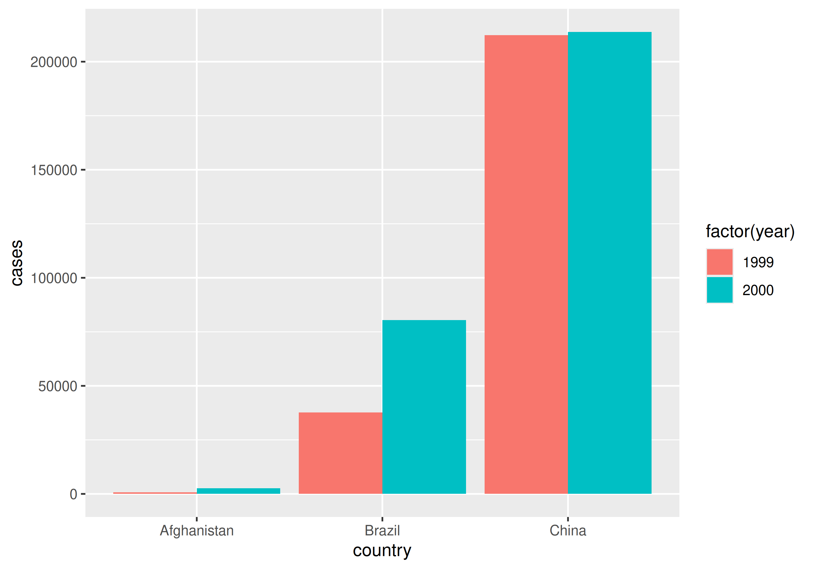
Why do we care?

country	1999	2000
Afghanistan	745	2666
Brazil	37737	80488
China	212258	213766
Tuberculosis cases per year per country

How would you plot this untidy data as the number of cases by country for each year?

ggplot(data = table4a, aes(x = ???, y = ???)) + 
  ???

Note

table4a is a built-in data frame
Type table4a in the console to take a look
Type ?table4a to pull up the help file with information

Why do we care?

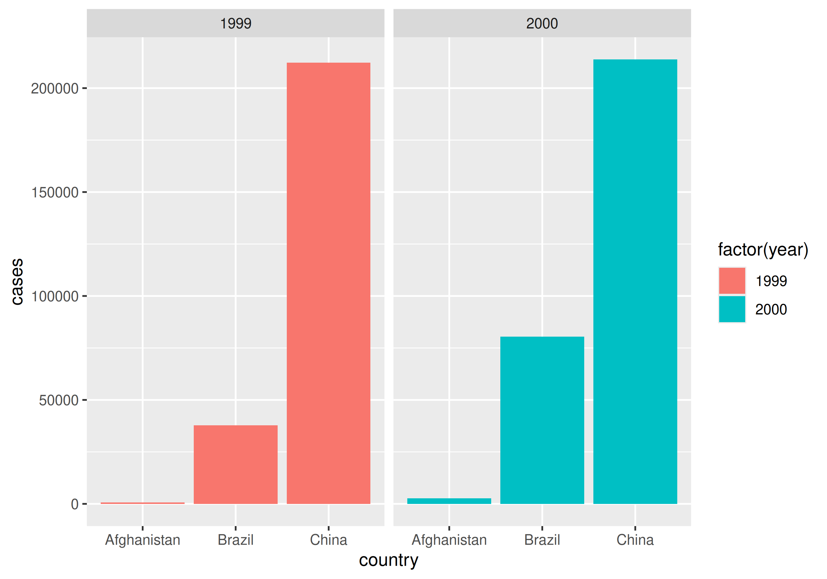
With un-tidy data

ggplot(data = table4a, aes(x = country, y = `1999`)) +
  geom_bar(stat = "identity", fill = "blue")

ggplot(data = table4a, aes(x = country, y = `2000`)) +
  geom_bar(stat = "identity", fill = "red")

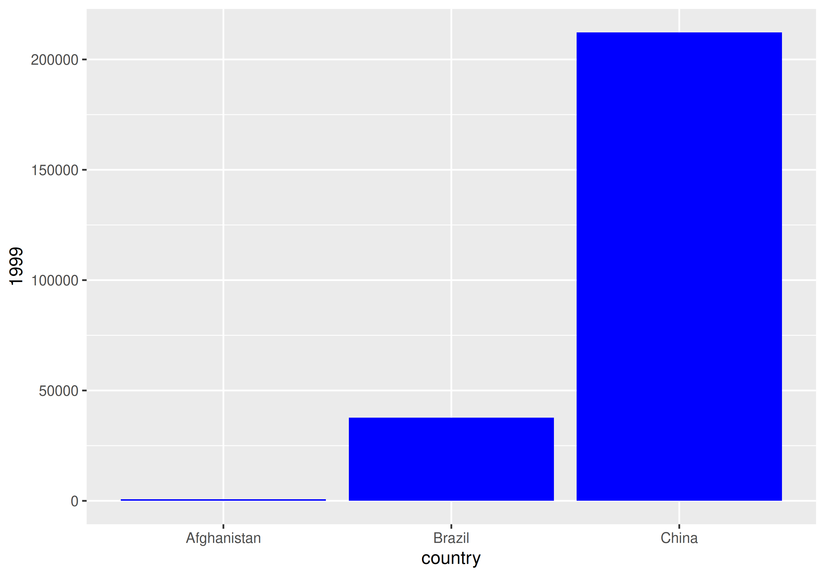
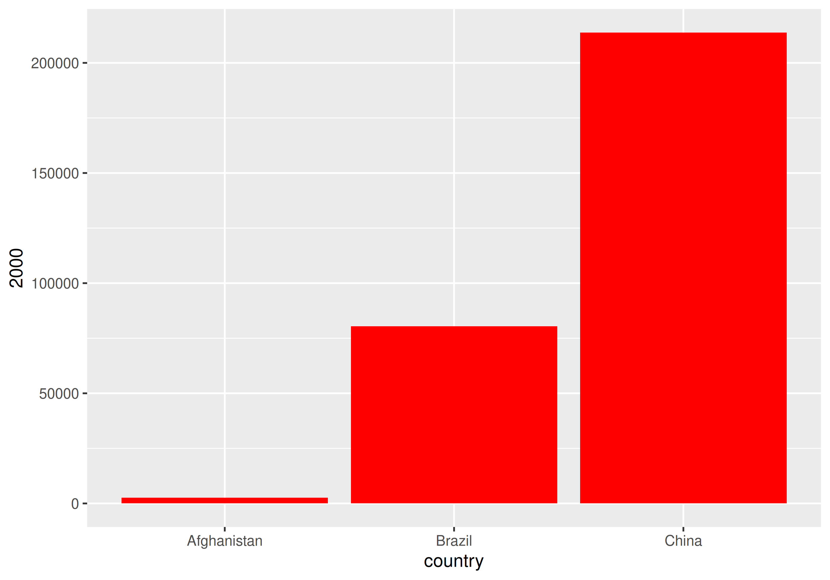
We have to plot it twice!

Why do we care?

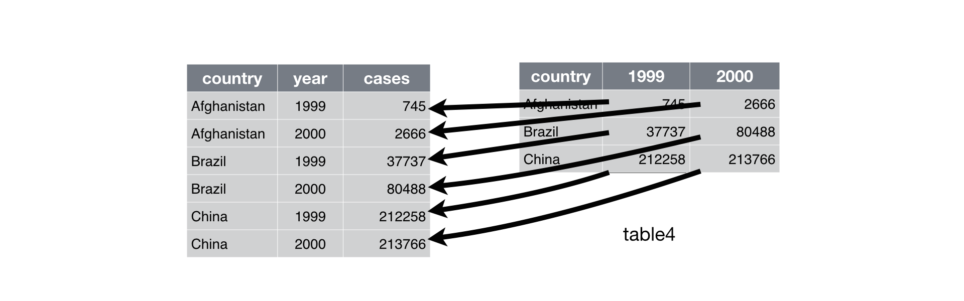
With tidy data

country	year	cases	population
Afghanistan	1999	745	19987071
Afghanistan	2000	2666	20595360
Brazil	1999	37737	172006362
Brazil	2000	80488	174504898
China	1999	212258	1272915272
China	2000	213766	1280428583

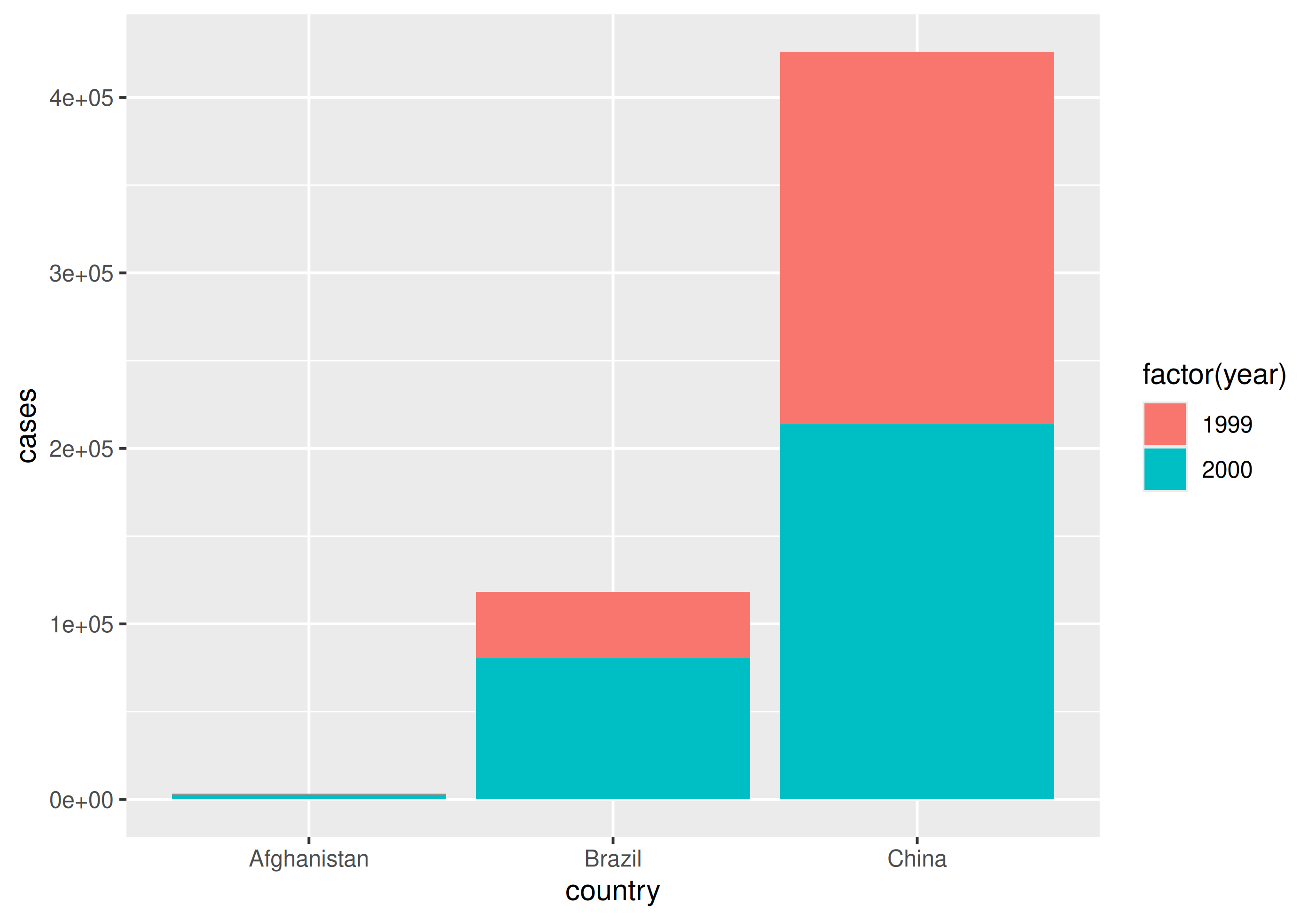
ggplot(data = table1, aes(x = country, y = cases, fill = factor(year))) +
  geom_bar(stat = "identity")

Why do we care?

With tidy data

ggplot(data = table1, 
       aes(x = country, y = cases, fill = factor(year))) +
  geom_bar(stat = "identity", position = "dodge")

ggplot(data = table1, 
       aes(x = country, y = cases, fill = factor(year))) +
  geom_bar(stat = "identity") + facet_wrap(~year)

Going long

`pivot_longer()`

A long data table next to a wide data table. The cells from the wide table are linked to cells in the long table by arrows

R for Data Science

Going long

From wide …

# A tibble: 114 × 6
   plot  depth coarse_silt medium_silt fine_silt total_silt
   <chr> <dbl>       <dbl>       <dbl>     <dbl>      <dbl>
 1 CSP01     4       14.1        11.2       8.17       33.5
 2 CSP01    12       14.1        11.7       9.03       34.8
 3 CSP01    35       10.3         9.51      7.47       27.3
 4 CSP01    53        9.4         9.1       8.7        27.2
 5 CSP01    83        9.79        8.79      7.29       25.9
 6 CSP01   105       10.8         9.4       8.22       28.4
 7 CSP08    10       16.3         9.55      6.23       32.1
 8 CSP08    27       14.3        10.4       6.1        30.8
 9 CSP08    90       15.1        11.5       7.56       34.2
10 CSP02     5       12.0        18.3      15.2        45.4
11 CSP02    11       10.7        18.3      14.3        43.3
12 CSP02    36       10.7        19.0      14.4        44.1
13 CSP02    56       11.1        18.0      13.7        42.8
14 CSP02    70       11.2        16.8      13.0        41  
15 CSP02    78        9.97       13.8      11.0        34.7
# ℹ 99 more rows

… to long

# A tibble: 456 × 4
   plot  depth type        amount
   <chr> <dbl> <chr>        <dbl>
 1 CSP01     4 coarse_silt  14.1 
 2 CSP01     4 medium_silt  11.2 
 3 CSP01     4 fine_silt     8.17
 4 CSP01     4 total_silt   33.5 
 5 CSP01    12 coarse_silt  14.1 
 6 CSP01    12 medium_silt  11.7 
 7 CSP01    12 fine_silt     9.03
 8 CSP01    12 total_silt   34.8 
 9 CSP01    35 coarse_silt  10.3 
10 CSP01    35 medium_silt   9.51
11 CSP01    35 fine_silt     7.47
12 CSP01    35 total_silt   27.3 
13 CSP01    53 coarse_silt   9.4 
14 CSP01    53 medium_silt   9.1 
15 CSP01    53 fine_silt     8.7 
16 CSP01    53 total_silt   27.2 
17 CSP01    83 coarse_silt   9.79
18 CSP01    83 medium_silt   8.79
19 CSP01    83 fine_silt     7.29
20 CSP01    83 total_silt   25.9 
# ℹ 436 more rows

Going long

`pivot_longer()` is from `tidyr`*

* part of the tidyverse

pivot_longer(data, cols = c(column1, column2),
             names_to = "new_categorical_column",
             values_to = "new_numerical_column")

tidyverse functions always start with data
Takes columns and converts to long data
Column names (column1 and column2) go into “new_categorical_column”
Column values (contents of column1 and column2) go into “new_numerical_column”

Hex logo for the tidyr R package

Going long

`pivot_longer()` is from `tidyr`*

* part of the tidyverse

pivot_longer(data, cols = c(column1, column2),
             names_to = "new_categorical_column",
             values_to = "new_numerical_column")

In our example:

data = size
cols = c(-plot, -depth, -habitat, -technician, -date)
- Here, easiest to exclude columns
names_to = "type"
values_to = "amount"

Hex logo for the tidyr R package

Going long

size_long <- pivot_longer(size, cols = c(-plot, -depth, -habitat, -technician, -date),
                          names_to = "type", values_to = "amount")

# A tibble: 1,026 × 7
   plot  depth habitat technician date       type        amount
   <chr> <dbl> <chr>   <chr>      <date>     <chr>        <dbl>
 1 CSP01     4 forest  Catharine  2009-04-23 coarse_sand  13.0 
 2 CSP01     4 forest  Catharine  2009-04-23 medium_sand  17.4 
 3 CSP01     4 forest  Catharine  2009-04-23 fine_sand    19.7 
 4 CSP01     4 forest  Catharine  2009-04-23 coarse_silt  14.1 
 5 CSP01     4 forest  Catharine  2009-04-23 medium_silt  11.2 
 6 CSP01     4 forest  Catharine  2009-04-23 fine_silt     8.17
 7 CSP01     4 forest  Catharine  2009-04-23 clay         16.3 
 8 CSP01     4 forest  Catharine  2009-04-23 total_sand   50.1 
 9 CSP01     4 forest  Catharine  2009-04-23 total_silt   33.5 
10 CSP01    12 forest  Catharine  2009-04-23 coarse_sand  10.7 
11 CSP01    12 forest  Catharine  2009-04-23 medium_sand  16.9 
12 CSP01    12 forest  Catharine  2009-04-23 fine_sand    19.2 
# ℹ 1,014 more rows

Your turn: Lengthen data

We’ll first create a summary dataset for sand variables

sand_sum <- read_csv("data/grain_size2.csv") |>
  mutate(total_sand = coarse_sand + medium_sand + fine_sand) |>
  group_by(plot) |>
  summarize(sample_size = n(),
            mean_sand = mean(total_sand),
            sd_sand = sd(total_sand),
            se_sand = sd_sand / sqrt(sample_size))

sand_sum

# A tibble: 27 × 5
   plot  sample_size mean_sand sd_sand se_sand
   <chr>       <int>     <dbl>   <dbl>   <dbl>
 1 CSP01           6      49.8   2.96    1.21 
 2 CSP02           7      34.7  10.8     4.06 
 3 CSP03           4      29.9   4.89    2.45 
 4 CSP04           5      30.3   2.18    0.973
 5 CSP05           5      44.6   5.52    2.47 
 6 CSP06           5      37.8   4.10    1.83 
 7 CSP07           3      36.6   7.30    4.21 
 8 CSP08           3      49.4   0.176   0.102
 9 CSP09           5      37.9   2.98    1.33 
10 CSP10           3      34.6   9.71    5.61 
# ℹ 17 more rows

Your turn: Lengthen data

Gather all variables except plot and sample_size into a long format

sand_long <- pivot_longer(sand_sum, 
                          cols = ???,
                          names_to = ???,
                          values_to = ???)

Going wide

`pivot_wider()`

A long data table next to a wide data table. The cells from the long table are linked to cells in the wide table by arrows

R for Data Science

Going wide

From long …

# A tibble: 456 × 4
   plot  depth type        amount
   <chr> <dbl> <chr>        <dbl>
 1 CSP01     4 coarse_silt  14.1 
 2 CSP01     4 medium_silt  11.2 
 3 CSP01     4 fine_silt     8.17
 4 CSP01     4 total_silt   33.5 
 5 CSP01    12 coarse_silt  14.1 
 6 CSP01    12 medium_silt  11.7 
 7 CSP01    12 fine_silt     9.03
 8 CSP01    12 total_silt   34.8 
 9 CSP01    35 coarse_silt  10.3 
10 CSP01    35 medium_silt   9.51
11 CSP01    35 fine_silt     7.47
12 CSP01    35 total_silt   27.3 
13 CSP01    53 coarse_silt   9.4 
14 CSP01    53 medium_silt   9.1 
15 CSP01    53 fine_silt     8.7 
16 CSP01    53 total_silt   27.2 
17 CSP01    83 coarse_silt   9.79
18 CSP01    83 medium_silt   8.79
19 CSP01    83 fine_silt     7.29
20 CSP01    83 total_silt   25.9 
# ℹ 436 more rows

… to wide

# A tibble: 114 × 6
   plot  depth coarse_silt medium_silt fine_silt total_silt
   <chr> <dbl>       <dbl>       <dbl>     <dbl>      <dbl>
 1 CSP01     4       14.1        11.2       8.17       33.5
 2 CSP01    12       14.1        11.7       9.03       34.8
 3 CSP01    35       10.3         9.51      7.47       27.3
 4 CSP01    53        9.4         9.1       8.7        27.2
 5 CSP01    83        9.79        8.79      7.29       25.9
 6 CSP01   105       10.8         9.4       8.22       28.4
 7 CSP08    10       16.3         9.55      6.23       32.1
 8 CSP08    27       14.3        10.4       6.1        30.8
 9 CSP08    90       15.1        11.5       7.56       34.2
10 CSP02     5       12.0        18.3      15.2        45.4
11 CSP02    11       10.7        18.3      14.3        43.3
12 CSP02    36       10.7        19.0      14.4        44.1
13 CSP02    56       11.1        18.0      13.7        42.8
14 CSP02    70       11.2        16.8      13.0        41  
15 CSP02    78        9.97       13.8      11.0        34.7
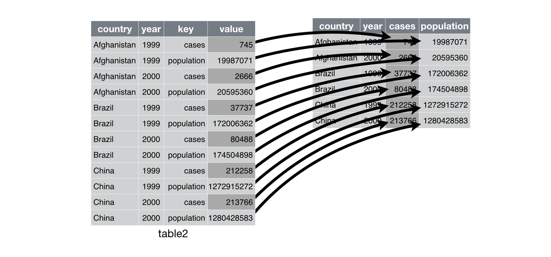
# ℹ 99 more rows

Going wide

`pivot_wider()` is from `tidyr`*

* part of the tidyverse

pivot_wider(data,
            names_from = existing_categorical_column,
            values_from = existing_numerical_column)

tidyverse functions always start with data
Takes columns and converts to wide data
Values in existing_categorical_column become column names
Values in existing_numerical_column become column contents

Hex logo for the tidyr R package

In our example:

data = size_long
names_from = type
values_from = amount

Going wide

size_wide <- pivot_wider(size_long, names_from = type, values_from = amount)

# A tibble: 114 × 14
   plot  depth habitat   technician date       coarse_sand medium_sand fine_sand coarse_silt medium_silt fine_silt  clay total_sand total_silt
   <chr> <dbl> <chr>     <chr>      <date>           <dbl>       <dbl>     <dbl>       <dbl>       <dbl>     <dbl> <dbl>      <dbl>      <dbl>
 1 CSP01     4 forest    Catharine  2009-04-23       13.0        17.4      19.7        14.1        11.2       8.17  16.3       50.1       33.5
 2 CSP01    12 forest    Catharine  2009-04-23       10.7        16.9      19.2        14.1        11.7       9.03  18.4       46.8       34.8
 3 CSP01    35 forest    Catharine  2009-04-23       12.1        17.8      16.1        10.3         9.51      7.47  26.7       46         27.3
 4 CSP01    53 forest    Catharine  2009-04-23       17.6        18.2      14.3         9.4         9.1       8.7   22.7       50.1       27.2
 5 CSP01    83 forest    Catharine  2009-04-23       21.0        18.4      14.3         9.79        8.79      7.29  20.4       53.8       25.9
 6 CSP01   105 forest    Catharine  2009-04-23       19.0        18.4      14.4        10.8         9.4       8.22  19.7       51.9       28.4
 7 CSP08    10 grassland Catharine  2009-03-02       11.6        17.1      20.8        16.3         9.55      6.23  18.4       49.6       32.1
 8 CSP08    27 grassland Catharine  2009-03-02       15.4        16.2      17.8        14.3        10.4       6.1   19.6       49.5       30.8
 9 CSP08    90 grassland Catharine  2009-03-02       14.9        15.8      18.6        15.1        11.5       7.56  16.5       49.2       34.2
10 CSP02     5 forest    Catharine  2009-05-06        8.75        8.64      8.66       12.0        18.3      15.2   28.5       26.0       45.4
# ℹ 104 more rows

Again: Why transpose?

Figures: Long data are great for graphing

size_long <- pivot_longer(size, cols = c(-plot, -depth, -technician, -habitat, -date),
                          names_to = "type", values_to = "amount")

ggplot(data = size_long, aes(y = depth, x = amount, colour = type)) +
  geom_point() +
  scale_y_reverse() +
  facet_wrap(~ type, nrow = 2)

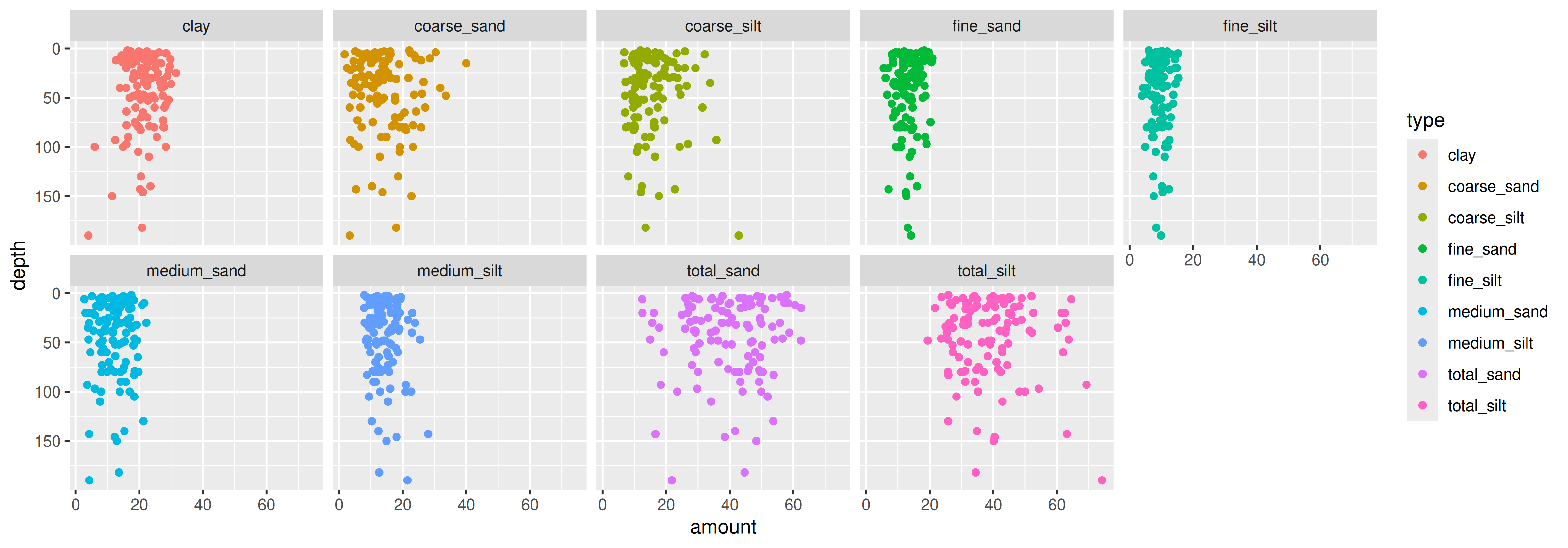
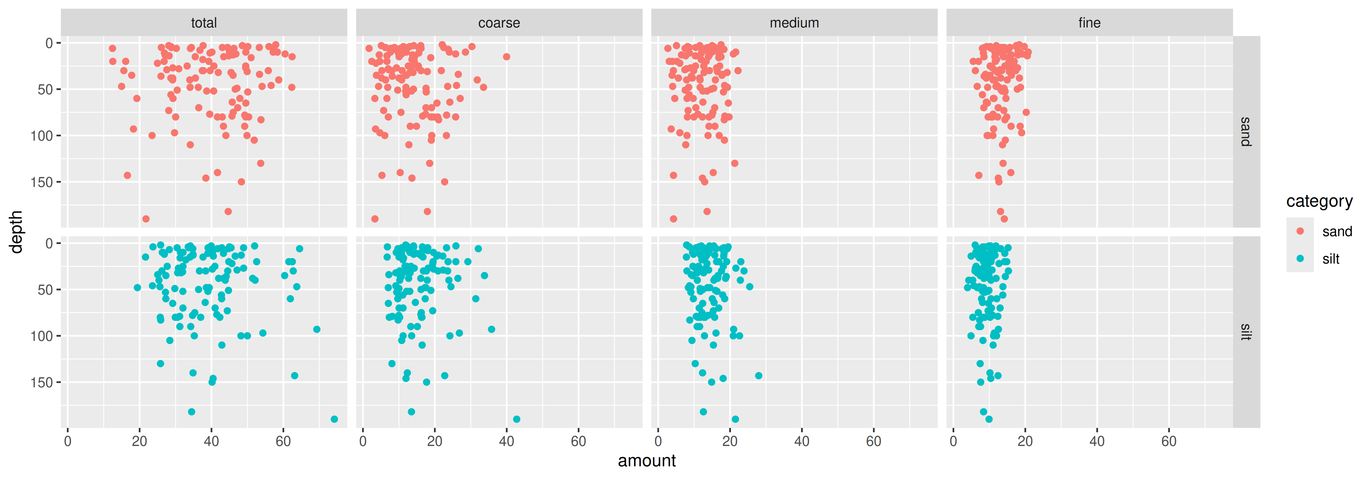
Again: Why transpose?

Figures: Take it to the next step

size <- read_csv("data/grain_size2.csv") |>
  left_join(meta, by = "plot") |>
  mutate(total_sand = coarse_sand + medium_sand + fine_sand,
         total_silt = coarse_silt + medium_silt + fine_silt)

size_long <- pivot_longer(size, cols = c(-plot, -depth, -technician, -habitat, -date, -clay),
                          names_to = c("size", "category"), values_to = "amount",
                          names_sep = "_") |>
  mutate(size = factor(size, levels = c("total", "coarse", "medium", "fine")))

# A tibble: 912 × 9
   plot  depth  clay habitat technician date       size   category amount
   <chr> <dbl> <dbl> <chr>   <chr>      <date>     <fct>  <chr>     <dbl>
 1 CSP01     4  16.3 forest  Catharine  2009-04-23 coarse sand      13.0 
 2 CSP01     4  16.3 forest  Catharine  2009-04-23 medium sand      17.4 
 3 CSP01     4  16.3 forest  Catharine  2009-04-23 fine   sand      19.7 
 4 CSP01     4  16.3 forest  Catharine  2009-04-23 coarse silt      14.1 
 5 CSP01     4  16.3 forest  Catharine  2009-04-23 medium silt      11.2 
 6 CSP01     4  16.3 forest  Catharine  2009-04-23 fine   silt       8.17
 7 CSP01     4  16.3 forest  Catharine  2009-04-23 total  sand      50.1 
 8 CSP01     4  16.3 forest  Catharine  2009-04-23 total  silt      33.5 
 9 CSP01    12  18.4 forest  Catharine  2009-04-23 coarse sand      10.7 
10 CSP01    12  18.4 forest  Catharine  2009-04-23 medium sand      16.9 
# ℹ 902 more rows

Again: Why transpose?

Figures: Take it to the next step

ggplot(data = size_long, 
       aes(y = depth, x = amount, colour = category)) +
  geom_point() +
  scale_y_reverse() +
  facet_grid(category ~ size)

Again: Why transpose?

Anlyses: Linear models `lm(y ~ x, data)`

Use pivot_longer() in analysis where grouping variables are important

i.e., do amounts of different size classes differ with depth? (need size classes in “type” column)

lm(amount ~ type + depth, data = size_long)

Use pivot_wider() in analyses where each variable must be in it’s own column

i.e., does the amount of sand differ with depth? (need size classes in separate columns)

lm(total_sand ~ depth, data = size_wide)

If you can’t figure out how to plot or analyse your data, they probably need to be transposed

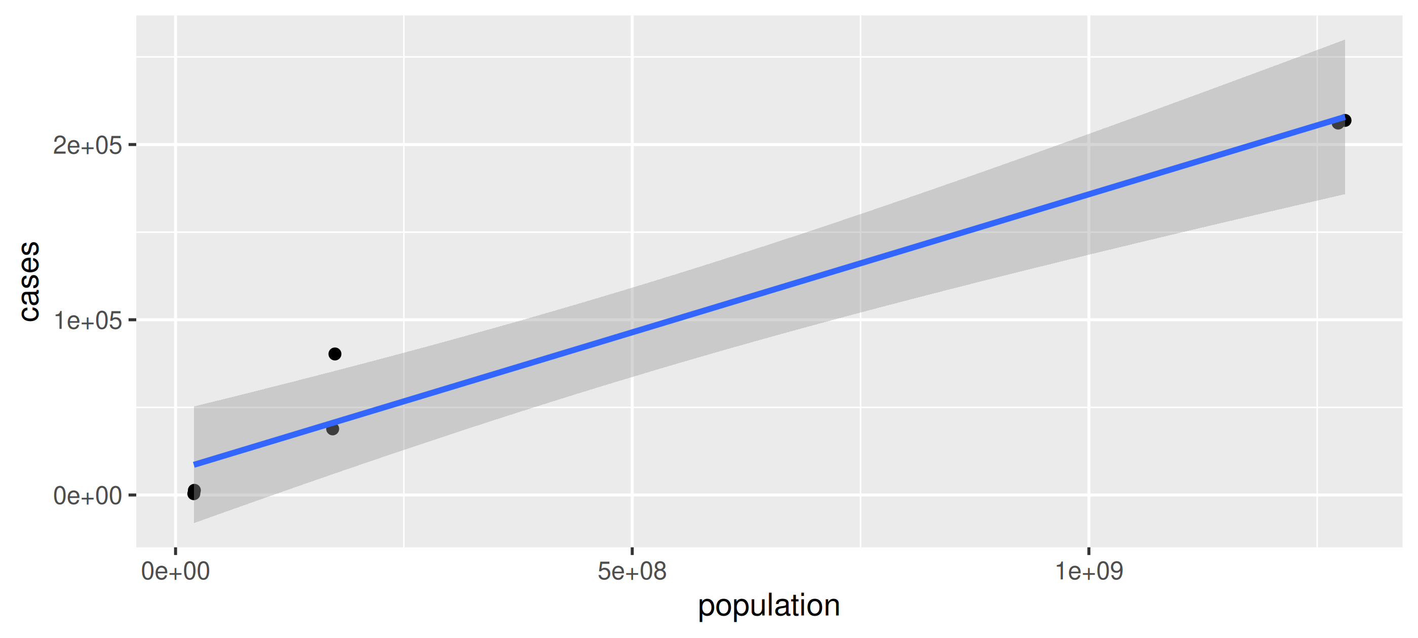
Your Turn: Transpose for plotting

Plot the number of Tuberculosis cases vs. the population in data frame table2

temp <- pivot_???(table2, ???)                    

ggplot(data = temp, ???) +    
  ???

Put it all together

meta <- read_csv("data/grain_meta.csv")

size <- read_csv("data/grain_size2.csv") |>
  left_join(meta, by = "plot") |>
  mutate(total_sand = coarse_sand + medium_sand + fine_sand,
         total_silt = coarse_silt + medium_silt + fine_silt)

size_sum <- size |>
  group_by(plot, habitat) |>
  summarize(sample_size = n(),
            total_sand = sum(total_sand),
            mean_sand = mean(total_sand),
            sd_sand = sd(total_sand),
            se_sand = sd_sand / sqrt(sample_size),
            total_silt = sum(total_silt),
            mean_silt = mean(total_silt),
            sd_silt = sd(total_silt),
            se_silt = sd_silt / sqrt(sample_size))

size_long <- size |>
  pivot_longer(cols = c(-plot, -depth, -technician, -habitat, -date, -clay), 
               values_to = "amount", names_to = c("size", "category"), names_sep = "_") |>
  mutate(size = factor(size, levels = c("total", "coarse", "medium", "fine")))

Put it all together

Save your data

write_csv(size, "datasets/size_total.csv")
write_csv(size_sum, "datasets/size_summary.csv")
write_csv(size_long, "datasets/size_long.csv")

Keep yourself organized

Keep your R-created data in a different folder from your ‘raw’ data
If you have a lot going on, split your work into several scripts, and number the both the scripts AND the data sets produced:
1_cleaned.csv
2_summarized.csv
3_graphing.csv

Wrapping up: Common mistakes

select() doesn’t work
- You may have the MASS package loaded, it also has a select() function
- Make sure you loaded tidyverse or dplyr packages
- Try using dplyr::select()
I can’t figure out how to pivot_wider() my data in the way I want it
- Sometimes you need to pivot_longer() before you can widen it
mutate() is giving me weird results
- Is your data grouped when it shouldn’t be?
- Try using ungroup() first
I get a warning when I join data sets
- Can be because multiple joins
- Can be because mismatched factor levels
  - If the category levels in one data frame do not match the other data frame
  - They will be transformed to character
  - If that’s a problem, use as.factor() to turn them back

Wrapping up: Further reading

R for Data Science
RStudio Data Manipulation with dplyr
- Or Help > Cheatsheets > Data Transformation with dplyr

Summarizing & Transforming Data in R

Saving you time and sanity

First things first

Types of Modifications

1. Subset

2. Joining data sets

3. Creating new columns

4. Summarize existing columns

5. Transpose

Getting ready

Check out the data:

Using data sets:

Subsetting

filter() observations

filter() is from dplyr*

filter() observations

filter() by category

filter() observations

filter() by measures

filter() observations

filter() by a combination use comma for AND

Equivalent to using &

Tangent

Logical Operators

Possible options

select() variables

select() is from dplyr*

select() variables

select() by name

Using helper functions

select() variables

Put it all together

To explore the data

To save as a separate object

Your turn: Subsetting

Joining or Merging data

Joining data sets

Measurements

Metadata

Joining them together

Joining data sets

Index or Metadata

Measurements

Types of Join: Which rows to keep?

left_join(x, y)

right_join(x, y)

inner_join(x, y)

full_join(x, y)

Joining data sets

left_join() is from dplyr*

Joining data sets

Keep all measurements (size), only keep meta if we have a measurement

Creating/modifying columns with mutate()

Creating new columns

mutate() is from dplyr*

Creating new columns

Tangent

Tangent: Vectorized

For example

For example

Back to mutate()…

Your turn: Creating new columns

Tangent

Where are…

… the decimal points?

… my data?

To see raw data

To see all rows

Back to mutate()…

Mutating by group

group_by() and ungroup() are from dplyr*

Mutating by group

mutate() without grouping

Grouping via group_by():

Your turn: Mutating by group

Put it all together

Check it out

Summarizing

Summarizing by group

summarize() is from dplyr*

`filter()` observations

`filter()` is from `dplyr`*

`filter()` observations

`filter()` by category

`filter()` observations

`filter()` by measures

`filter()` observations

`filter()` by a combination use comma for AND

`select()` variables

`select()` is from `dplyr`*

`select()` variables

`select()` by name

`select()` variables

`left_join(x, y)`

`right_join(x, y)`

`inner_join(x, y)`

`full_join(x, y)`

`left_join()` is from `dplyr`*

Keep all measurements (`size`), only keep `meta` if we have a measurement

Creating/modifying columns with `mutate()`

`mutate()` is from `dplyr`*

Back to `mutate()`…

Back to `mutate()`…

`group_by()` and `ungroup()` are from `dplyr`*

`mutate()` without grouping

Grouping via `group_by()`:

`summarize()` is from `dplyr`*

`mutate()`

`summarize()`

`n()` is from `dplyr`*

`pivot_longer()`

`pivot_longer()` is from `tidyr`*

`pivot_longer()` is from `tidyr`*

`pivot_wider()`

`pivot_wider()` is from `tidyr`*

Anlyses: Linear models `lm(y ~ x, data)`