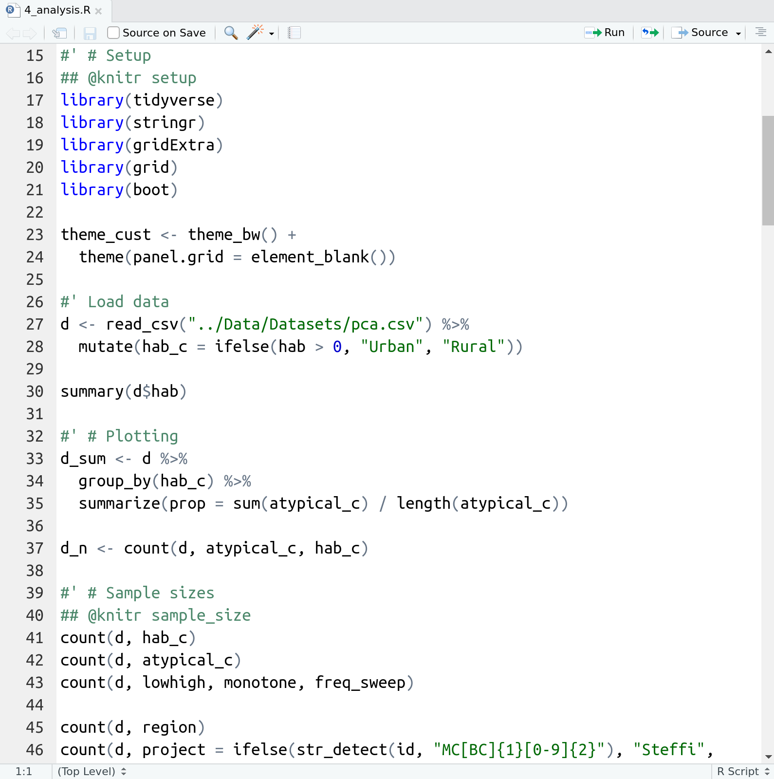
56 * 5.8[1] 324.8
steffilazerte
@steffilazerte@fosstodon.org
steffilazerte.ca

Compiled: 2025-10-27

Artwork by @allison_horst
A programming language is a way to give instructions in order to get a computer to do something
R, what is 56 times 5.8?
![]()

We’re using weathercan today
![]()
![]()
We’re using both RStudio and R today


Moral of the story?
Make friends, code in groups, learn together and don’t beat yourself up

Artwork by @allison_horst

1library(weathercan)
2stations()
3stations_search("Brandon")
4w <- weather_dl("49909", start = "2025-09-01")
5n <- normals_dl("5010480")library() function
stations() function to get a list of stations
stations_search() function to search for a station
weather_dl() to download recent data by station_id
normals_dl() to download climate normals by climate_id
That’s it! Workshop over 😁
?weather_dlTo cite 'weathercan' in publications, please use:
LaZerte, Stefanie E and Sam Albers (2018). weathercan: Download and format weather data from Environment
and Climate Change Canada. The Journal of Open Source Software 3(22):571. doi:10.21105/joss.00571.
A BibTeX entry for LaTeX users is
@Article{,
title = {{weathercan}: {D}ownload and format weather data from Environment and Climate Change Canada},
author = {Stefanie E LaZerte and Sam Albers},
journal = {The Journal of Open Source Software},
volume = {3},
number = {22},
pages = {571},
year = {2018},
url = {https://joss.theoj.org/papers/10.21105/joss.00571},
}flagsglossaryglossary_normals# A tibble: 16 × 2
code meaning
<chr> <chr>
1 A Accumulated
2 B More than one occurrence and estimated
3 C Precipitation occurred, amount uncertain
4 D Data subject to further quality control procedure
5 E Estimated
6 F Accumulated and estimated
7 L Precipitation may or may not have occurred
8 M Missing
9 N Temperature missing but known to be > 0
10 S More than one occurrence
11 T Trace
12 Y Temperature missing but known to be < 0
13 [empty] Indicates an unobserved value
14 ^ The value displayed is based on incomplete data
15 † Data that is not subject to review by the National Climate Archives
16 <NA> Not Available Where?
stations()# A tibble: 26,451 × 17
prov station_name station_id climate_id WMO_id TC_id lat lon elev tz interval start end normals
<chr> <chr> <dbl> <chr> <dbl> <chr> <dbl> <dbl> <dbl> <chr> <chr> <dbl> <dbl> <lgl>
1 AB DAYSLAND 1795 301AR54 NA <NA> 52.9 -112. 689. Etc/GMT+7 day 1908 1922 FALSE
2 AB DAYSLAND 1795 301AR54 NA <NA> 52.9 -112. 689. Etc/GMT+7 hour NA NA FALSE
3 AB DAYSLAND 1795 301AR54 NA <NA> 52.9 -112. 689. Etc/GMT+7 month 1908 1922 FALSE
4 AB EDMONTON CORONATION 1796 301BK03 NA <NA> 53.6 -114. 671. Etc/GMT+7 day 1978 1979 FALSE
5 AB EDMONTON CORONATION 1796 301BK03 NA <NA> 53.6 -114. 671. Etc/GMT+7 hour NA NA FALSE
6 AB EDMONTON CORONATION 1796 301BK03 NA <NA> 53.6 -114. 671. Etc/GMT+7 month 1978 1979 FALSE
7 AB FLEET 1797 301B6L0 NA <NA> 52.2 -112. 838. Etc/GMT+7 day 1987 1990 FALSE
8 AB FLEET 1797 301B6L0 NA <NA> 52.2 -112. 838. Etc/GMT+7 hour NA NA FALSE
9 AB FLEET 1797 301B6L0 NA <NA> 52.2 -112. 838. Etc/GMT+7 month 1987 1990 FALSE
10 AB GOLDEN VALLEY 1798 301B8LR NA <NA> 53.2 -110. 640 Etc/GMT+7 day 1987 1998 FALSE
# ℹ 26,441 more rows
# ℹ 3 more variables: normals_1991_2020 <lgl>, normals_1981_2010 <lgl>, normals_1971_2000 <lgl>stations_dl()According to Environment Canada, Modified Date: 2025-10-08 23:30 UTCEnvironment Canada Disclaimers:
"Station Inventory Disclaimer: Please note that this inventory list is a snapshot of stations on our website as of the modified date, and may be subject to change without notice."
"Station ID Disclaimer: Station IDs are an internal index numbering system and may be subject to change without notice."Stations data saved...
Use `stations()` to access most recent version and `stations_meta()` to see when this was last updatedstations_search()# A tibble: 17 × 17
prov station_name station_id climate_id WMO_id TC_id lat lon elev tz interval start end normals
<chr> <chr> <dbl> <chr> <dbl> <chr> <dbl> <dbl> <dbl> <chr> <chr> <dbl> <dbl> <lgl>
1 MB BRANDON #1 WINTER BAY 3474 5010498 NA <NA> 49.8 -100.0 396 Etc/G… day 1987 2002 FALSE
2 MB BRANDON #1 WINTER BAY 3474 5010498 NA <NA> 49.8 -100.0 396 Etc/G… month 1987 2002 FALSE
3 MB BRANDON A 3471 5010480 71140 YBR 49.9 -100.0 409. Etc/G… day 1941 2012 TRUE
4 MB BRANDON A 3471 5010480 71140 YBR 49.9 -100.0 409. Etc/G… hour 1958 2012 TRUE
5 MB BRANDON A 3471 5010480 71140 YBR 49.9 -100.0 409. Etc/G… month 1941 2012 TRUE
6 MB BRANDON CDA 3472 5010485 NA <NA> 49.9 -100.0 363. Etc/G… day 1890 2010 TRUE
7 MB BRANDON CDA 3472 5010485 NA <NA> 49.9 -100.0 363. Etc/G… month 1890 2007 TRUE
8 MB BRANDON MUNI A 50821 5010481 71140 YBR 49.9 -100.0 409. Etc/G… day 2012 2025 TRUE
9 MB BRANDON MUNI A 50821 5010481 71140 YBR 49.9 -100.0 409. Etc/G… hour 2012 2025 TRUE
10 MB BRANDON MUNI A 55738 5010482 71140 YBR 49.9 -100.0 409. Etc/G… day 2025 2025 FALSE
11 MB BRANDON MUNI A 55738 5010482 71140 YBR 49.9 -100.0 409. Etc/G… hour 2025 2025 FALSE
12 MB BRANDON RCS 49909 5010490 71136 PBO 49.9 -100.0 409. Etc/G… day 2012 2025 FALSE
13 MB BRANDON RCS 49909 5010490 71136 PBO 49.9 -100.0 409. Etc/G… hour 2012 2025 FALSE
14 MB BRANDON SOUTH 3473 5010494 NA <NA> 49.8 -100.0 396. Etc/G… day 1972 1975 FALSE
15 MB BRANDON SOUTH 3473 5010494 NA <NA> 49.8 -100.0 396. Etc/G… month 1972 1975 FALSE
16 QC ST GABRIEL DE BRANDON 5273 7017270 NA <NA> 46.3 -73.4 198. Etc/G… day 1919 1985 FALSE
17 QC ST GABRIEL DE BRANDON 5273 7017270 NA <NA> 46.3 -73.4 198. Etc/G… month 1919 1985 FALSE
# ℹ 3 more variables: normals_1991_2020 <lgl>, normals_1981_2010 <lgl>, normals_1971_2000 <lgl>stations_search()# A tibble: 2 × 17
prov station_name station_id climate_id WMO_id TC_id lat lon elev tz interval start end normals
<chr> <chr> <dbl> <chr> <dbl> <chr> <dbl> <dbl> <dbl> <chr> <chr> <dbl> <dbl> <lgl>
1 MB BRANDON MUNI A 50821 5010481 71140 YBR 49.9 -100.0 409. Etc/GMT+6 day 2012 2025 TRUE
2 MB BRANDON RCS 49909 5010490 71136 PBO 49.9 -100.0 409. Etc/GMT+6 day 2012 2025 FALSE
# ℹ 3 more variables: normals_1991_2020 <lgl>, normals_1981_2010 <lgl>, normals_1971_2000 <lgl>Hmmm, that’s a bit tough to read
glimpse() from the dplyr packagestations_search(
name = "Brandon",
interval = "day",
starts_latest = 2020,
ends_earliest = 2025
) |> dplyr::glimpse()Rows: 2
Columns: 17
$ prov <chr> "MB", "MB"
$ station_name <chr> "BRANDON MUNI A", "BRANDON RCS"
$ station_id <dbl> 50821, 49909
$ climate_id <chr> "5010481", "5010490"
$ WMO_id <dbl> 71140, 71136
$ TC_id <chr> "YBR", "PBO"
$ lat <dbl> 49.91, 49.90
$ lon <dbl> -99.95, -99.95
$ elev <dbl> 409.3, 409.4
$ tz <chr> "Etc/GMT+6", "Etc/GMT+6"
$ interval <chr> "day", "day"
$ start <dbl> 2012, 2012
$ end <dbl> 2025, 2025
$ normals <lgl> TRUE, FALSE
$ normals_1991_2020 <lgl> TRUE, FALSE
$ normals_1981_2010 <lgl> FALSE, FALSE
$ normals_1971_2000 <lgl> FALSE, FALSEAfter running this code, click on ‘s’ in the Environment Pane
stations_search()# A tibble: 15 × 18
prov station_name station_id climate_id WMO_id TC_id lat lon elev tz interval start end normals
<chr> <chr> <dbl> <chr> <dbl> <chr> <dbl> <dbl> <dbl> <chr> <chr> <dbl> <dbl> <lgl>
1 MB BRANDON SOUTH 3473 5010494 NA <NA> 49.8 -100.0 396. Etc/G… day 1972 1975 FALSE
2 MB BRANDON SOUTH 3473 5010494 NA <NA> 49.8 -100.0 396. Etc/G… month 1972 1975 FALSE
3 MB BRANDON CDA 3472 5010485 NA <NA> 49.9 -100.0 363. Etc/G… day 1890 2010 TRUE
4 MB BRANDON CDA 3472 5010485 NA <NA> 49.9 -100.0 363. Etc/G… month 1890 2007 TRUE
5 MB BRANDON #1 WINTER BAY 3474 5010498 NA <NA> 49.8 -100.0 396 Etc/G… day 1987 2002 FALSE
6 MB BRANDON #1 WINTER BAY 3474 5010498 NA <NA> 49.8 -100.0 396 Etc/G… month 1987 2002 FALSE
7 MB BRANDON RCS 49909 5010490 71136 PBO 49.9 -100.0 409. Etc/G… day 2012 2025 FALSE
8 MB BRANDON RCS 49909 5010490 71136 PBO 49.9 -100.0 409. Etc/G… hour 2012 2025 FALSE
9 MB BRANDON A 3471 5010480 71140 YBR 49.9 -100.0 409. Etc/G… day 1941 2012 TRUE
10 MB BRANDON A 3471 5010480 71140 YBR 49.9 -100.0 409. Etc/G… hour 1958 2012 TRUE
11 MB BRANDON A 3471 5010480 71140 YBR 49.9 -100.0 409. Etc/G… month 1941 2012 TRUE
12 MB BRANDON MUNI A 50821 5010481 71140 YBR 49.9 -100.0 409. Etc/G… day 2012 2025 TRUE
13 MB BRANDON MUNI A 50821 5010481 71140 YBR 49.9 -100.0 409. Etc/G… hour 2012 2025 TRUE
14 MB BRANDON MUNI A 55738 5010482 71140 YBR 49.9 -100.0 409. Etc/G… day 2025 2025 FALSE
15 MB BRANDON MUNI A 55738 5010482 71140 YBR 49.9 -100.0 409. Etc/G… hour 2025 2025 FALSE
# ℹ 4 more variables: normals_1991_2020 <lgl>, normals_1981_2010 <lgl>, normals_1971_2000 <lgl>, distance <dbl>stations_search()library(dplyr)
library(stringr)
stations() |>
filter(
str_detect(station_name, "BRANDON"),
interval == "day",
start <= 2020,
end >= 2025
)# A tibble: 2 × 17
prov station_name station_id climate_id WMO_id TC_id lat lon elev tz interval start end normals
<chr> <chr> <dbl> <chr> <dbl> <chr> <dbl> <dbl> <dbl> <chr> <chr> <dbl> <dbl> <lgl>
1 MB BRANDON RCS 49909 5010490 71136 PBO 49.9 -100.0 409. Etc/GMT+6 day 2012 2025 FALSE
2 MB BRANDON MUNI A 50821 5010481 71140 YBR 49.9 -100.0 409. Etc/GMT+6 day 2012 2025 TRUE
# ℹ 3 more variables: normals_1991_2020 <lgl>, normals_1981_2010 <lgl>, normals_1971_2000 <lgl>We’re not actually using
stations_search()at all here
Locate a station of interest, take note of it’s Station ID
(Feel free to locate several stations)
Historical hourly, daily,
or monthly weather
weather_dl()# A tibble: 8 × 17
prov station_name station_id climate_id WMO_id TC_id lat lon elev tz interval start end normals
<chr> <chr> <dbl> <chr> <dbl> <chr> <dbl> <dbl> <dbl> <chr> <chr> <dbl> <dbl> <lgl>
1 MB BRANDON #1 WINTER BAY 3474 5010498 NA <NA> 49.8 -100.0 396 Etc/GM… day 1987 2002 FALSE
2 MB BRANDON A 3471 5010480 71140 YBR 49.9 -100.0 409. Etc/GM… day 1941 2012 TRUE
3 MB BRANDON CDA 3472 5010485 NA <NA> 49.9 -100.0 363. Etc/GM… day 1890 2010 TRUE
4 MB BRANDON MUNI A 50821 5010481 71140 YBR 49.9 -100.0 409. Etc/GM… day 2012 2025 TRUE
5 MB BRANDON MUNI A 55738 5010482 71140 YBR 49.9 -100.0 409. Etc/GM… day 2025 2025 FALSE
6 MB BRANDON RCS 49909 5010490 71136 PBO 49.9 -100.0 409. Etc/GM… day 2012 2025 FALSE
7 MB BRANDON SOUTH 3473 5010494 NA <NA> 49.8 -100.0 396. Etc/GM… day 1972 1975 FALSE
8 QC ST GABRIEL DE BRANDON 5273 7017270 NA <NA> 46.3 -73.4 198. Etc/GM… day 1919 1985 FALSE
# ℹ 3 more variables: normals_1991_2020 <lgl>, normals_1981_2010 <lgl>, normals_1971_2000 <lgl>weathercan uses ‘caching’ and will only download this data once per session
# A tibble: 243 × 37
   station_name station_id station_operator prov    lat    lon  elev climate_id WMO_id TC_id date       year  month
   <chr>             <dbl> <lgl>            <chr> <dbl>  <dbl> <dbl> <chr>      <chr>  <chr> <date>     <chr> <chr>
 1 BRANDON RCS       49909 NA               MB     49.9 -100.0  409. 5010490    71136  PBO   2025-01-01 2025  01
 2 BRANDON RCS       49909 NA               MB     49.9 -100.0  409. 5010490    71136  PBO   2025-01-02 2025  01
 3 BRANDON RCS       49909 NA               MB     49.9 -100.0  409. 5010490    71136  PBO   2025-01-03 2025  01
 4 BRANDON RCS       49909 NA               MB     49.9 -100.0  409. 5010490    71136  PBO   2025-01-04 2025  01
 5 BRANDON RCS       49909 NA               MB     49.9 -100.0  409. 5010490    71136  PBO   2025-01-05 2025  01
 6 BRANDON RCS       49909 NA               MB     49.9 -100.0  409. 5010490    71136  PBO   2025-01-06 2025  01
 7 BRANDON RCS       49909 NA               MB     49.9 -100.0  409. 5010490    71136  PBO   2025-01-07 2025  01
 8 BRANDON RCS       49909 NA               MB     49.9 -100.0  409. 5010490    71136  PBO   2025-01-08 2025  01
 9 BRANDON RCS       49909 NA               MB     49.9 -100.0  409. 5010490    71136  PBO   2025-01-09 2025  01
10 BRANDON RCS       49909 NA               MB     49.9 -100.0  409. 5010490    71136  PBO   2025-01-10 2025  01
# ℹ 233 more rows
# ℹ 24 more variables: day <chr>, qual <chr>, cool_deg_days <dbl>, cool_deg_days_flag <chr>, dir_max_gust <dbl>,
#   dir_max_gust_flag <chr>, heat_deg_days <dbl>, heat_deg_days_flag <chr>, max_temp <dbl>, max_temp_flag <chr>,
#   mean_temp <dbl>, mean_temp_flag <chr>, min_temp <dbl>, min_temp_flag <chr>, snow_grnd <dbl>, snow_grnd_flag <chr>,
#   spd_max_gust <dbl>, spd_max_gust_flag <chr>, total_precip <dbl>, total_precip_flag <chr>, total_rain <dbl>,
#   total_rain_flag <chr>, total_snow <dbl>, total_snow_flag <chr>
A lot of stuff, apparently…
── Data Summary ────────────────────────
                           Values
Name                       w
Number of rows             243
Number of columns          37
_______________________
Column type frequency:
  character                20
  Date                     1
  logical                  1
  numeric                  15
________________________
Group variables            None

── Variable type: character ────────────────────────────────────────────────────────────────────────────────────────────
   skim_variable      n_missing complete_rate min max empty n_unique whitespace
 1 station_name               0        1       11  11     0        1          0
 2 prov                       0        1        2   2     0        1          0
 3 climate_id                 0        1        7   7     0        1          0
 4 WMO_id                     0        1        5   5     0        1          0
 5 TC_id                      0        1        3   3     0        1          0
 6 year                       0        1        4   4     0        1          0
 7 month                      0        1        2   2     0        8          0
 8 day                        0        1        2   2     0       31          0
 9 qual                     243        0       NA  NA     0        0          0
10 cool_deg_days_flag       236        0.0288   1   1     0        1          0
11 dir_max_gust_flag        236        0.0288   1   1     0        1          0
12 heat_deg_days_flag       236        0.0288   1   1     0        1          0
13 max_temp_flag            236        0.0288   1   1     0        1          0
14 mean_temp_flag           236        0.0288   1   1     0        1          0
15 min_temp_flag            236        0.0288   1   1     0        1          0
16 snow_grnd_flag           243        0       NA  NA     0        0          0
17 spd_max_gust_flag        236        0.0288   1   1     0        1          0
18 total_precip_flag        236        0.0288   1   1     0        1          0
19 total_rain_flag          243        0       NA  NA     0        0          0
20 total_snow_flag          243        0       NA  NA     0        0          0

── Variable type: Date ─────────────────────────────────────────────────────────────────────────────────────────────────
  skim_variable n_missing complete_rate min        max        median     n_unique
1 date                  0             1 2025-01-01 2025-08-31 2025-05-02      243

── Variable type: logical ──────────────────────────────────────────────────────────────────────────────────────────────
  skim_variable    n_missing complete_rate mean count
1 station_operator       243             0  NaN ": "

── Variable type: numeric ──────────────────────────────────────────────────────────────────────────────────────────────
   skim_variable n_missing complete_rate      mean    sd      p0      p25      p50       p75    p100 hist
 1 station_id            0         1     49909      0    49909   49909    49909    49909     49909   "▁▁▇▁▁"
 2 lat                   0         1        49.9    0       49.9    49.9     49.9     49.9      49.9 "▁▁▇▁▁"
 3 lon                   0         1      -100.0    0     -100.0  -100.0   -100.0   -100.0    -100.0 "▁▁▇▁▁"
 4 elev                  0         1       409.     0      409.    409.     409.     409.      409.  "▁▁▇▁▁"
 5 cool_deg_days         7         0.971     0.444  1.10     0       0        0        0         5.4 "▇▁▁▁▁"
 6 dir_max_gust         89         0.634    19.2   10.9      1       7       23       29        35   "▇▂▃▆▇"
 7 heat_deg_days         7         0.971    14.8   14.9      0       1.17     9.85    24.9      49.8 "▇▂▃▂▂"
 8 max_temp              7         0.971    10.1   16.2    -27.9    -1.65    15.6     24.1      32.9 "▂▂▅▅▇"
 9 mean_temp             7         0.971     3.64  15.3    -31.8    -6.9      8.15    16.8      23.4 "▂▂▃▃▇"
10 min_temp              7         0.971    -2.84  14.9    -37.1   -12.2      1.05     9.83     18.3 "▂▃▅▅▇"
11 snow_grnd           123         0.494    16.9   10.0      1       5       19       27        31   "▆▂▂▂▇"
12 spd_max_gust         89         0.634    42.8   10.1     31      35       40.5     48        76   "▇▅▂▁▁"
13 total_precip          7         0.971     0.936  3.57     0       0        0        0.125    43.5 "▇▁▁▁▁"
14 total_rain          243         0       NaN     NA       NA      NA       NA       NA        NA   " "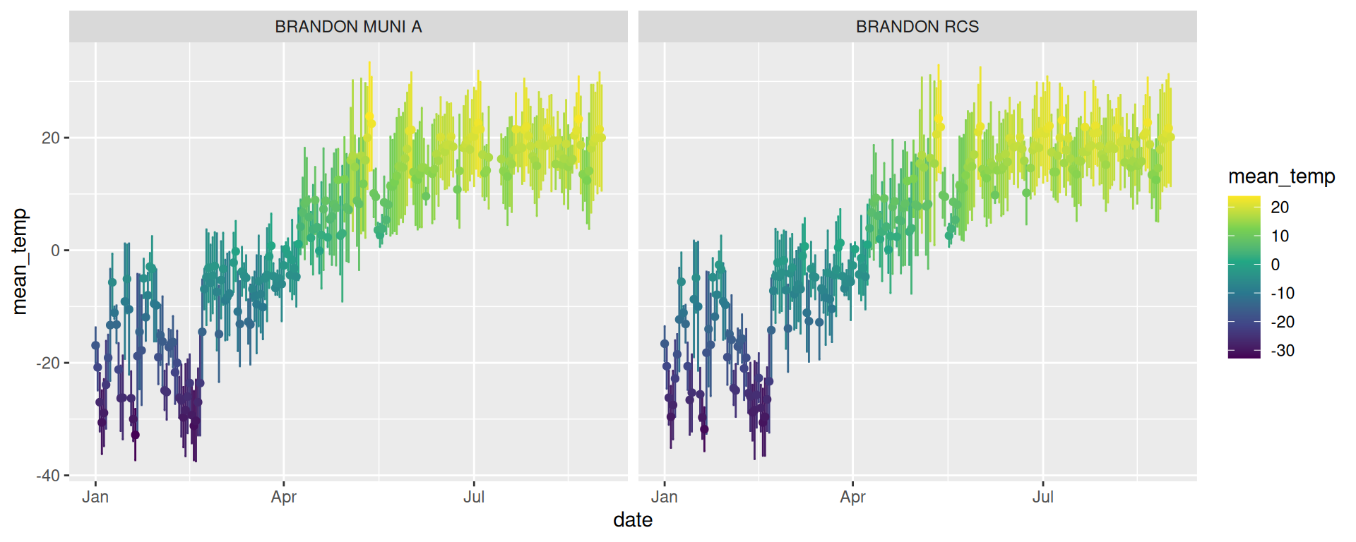
15 total_snow 243 0 NaN NA NA NA NA NA NA " " weather_dl()s <- stations_search("Brandon", interval = "day")
w <- weather_dl(station_id = s$station_id, interval = "day", start = "2025-01-01", end = "2025-08-31")There are no data for some stations (3474, 3471, 3472, 3473, 5273), in this time range (2025-01-01 to 2025-08-31), for this interval (day)
Available Station Data:
# A tibble: 11 × 17
prov station_name station_id climate_id WMO_id TC_id lat lon elev tz interval start end normals
<chr> <chr> <dbl> <chr> <dbl> <chr> <dbl> <dbl> <dbl> <chr> <chr> <dbl> <dbl> <lgl>
1 MB BRANDON A 3471 5010480 71140 YBR 49.9 -100.0 409. Etc/G… day 1941 2012 TRUE
2 MB BRANDON A 3471 5010480 71140 YBR 49.9 -100.0 409. Etc/G… hour 1958 2012 TRUE
3 MB BRANDON A 3471 5010480 71140 YBR 49.9 -100.0 409. Etc/G… month 1941 2012 TRUE
4 MB BRANDON CDA 3472 5010485 NA <NA> 49.9 -100.0 363. Etc/G… day 1890 2010 TRUE
5 MB BRANDON CDA 3472 5010485 NA <NA> 49.9 -100.0 363. Etc/G… month 1890 2007 TRUE
6 MB BRANDON SOUTH 3473 5010494 NA <NA> 49.8 -100.0 396. Etc/G… day 1972 1975 FALSE
7 MB BRANDON SOUTH 3473 5010494 NA <NA> 49.8 -100.0 396. Etc/G… month 1972 1975 FALSE
8 MB BRANDON #1 WINTER BAY 3474 5010498 NA <NA> 49.8 -100.0 396 Etc/G… day 1987 2002 FALSE
9 MB BRANDON #1 WINTER BAY 3474 5010498 NA <NA> 49.8 -100.0 396 Etc/G… month 1987 2002 FALSE
10 QC ST GABRIEL DE BRANDON 5273 7017270 NA <NA> 46.3 -73.4 198. Etc/G… day 1919 1985 FALSE
11 QC ST GABRIEL DE BRANDON 5273 7017270 NA <NA> 46.3 -73.4 198. Etc/G… month 1919 1985 FALSE
# ℹ 3 more variables: normals_1991_2020 <lgl>, normals_1981_2010 <lgl>, normals_1971_2000 <lgl>Some stations don’t have data in this time range (makes sense if you look at their start/end ranges)
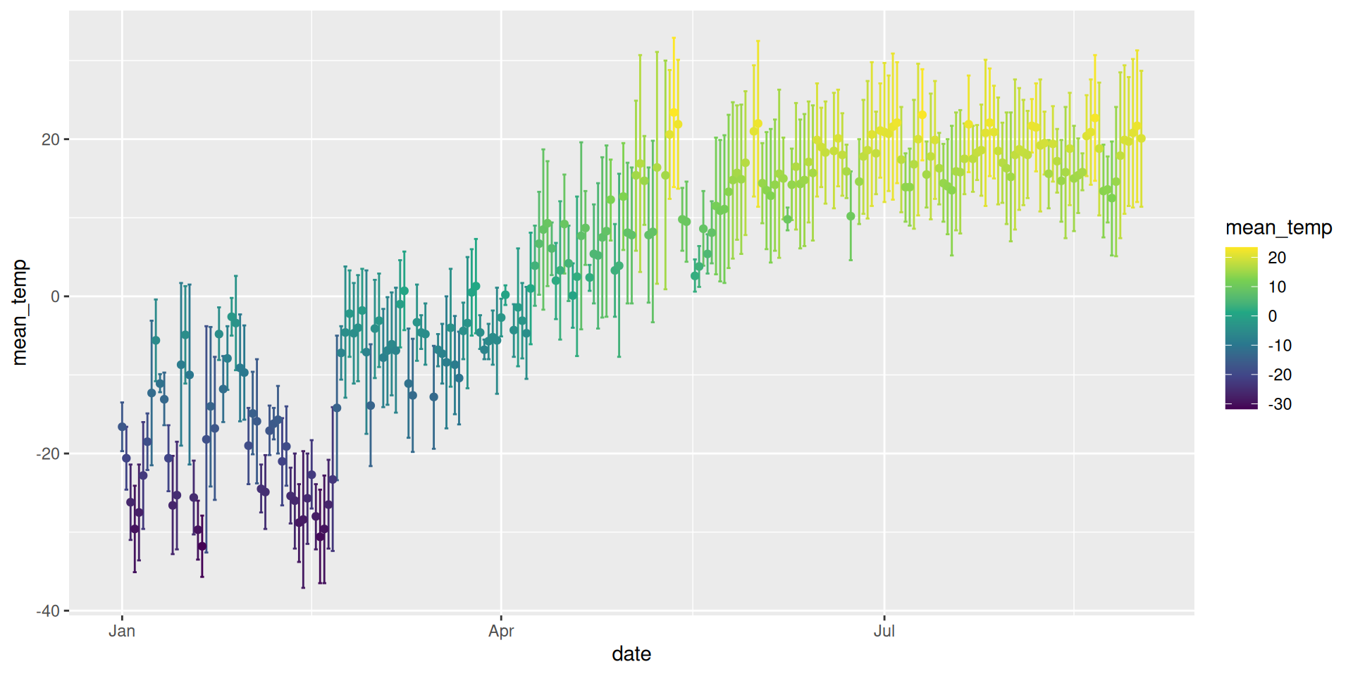
Download some data for your station(s).
Take a look at them!
Climate normals and averages
calculated by ECCC for 30-year periods
normals_dl()The most current normals available for download by weathercan are '1981-2010'# A tibble: 5 × 17
prov station_name station_id climate_id WMO_id TC_id lat lon elev tz interval start end normals
<chr> <chr> <dbl> <chr> <dbl> <chr> <dbl> <dbl> <dbl> <chr> <chr> <dbl> <dbl> <lgl>
1 MB BRANDON A 3471 5010480 71140 YBR 49.9 -100.0 409. Etc/GMT+6 day 1941 2012 TRUE
2 MB BRANDON A 3471 5010480 71140 YBR 49.9 -100.0 409. Etc/GMT+6 hour 1958 2012 TRUE
3 MB BRANDON A 3471 5010480 71140 YBR 49.9 -100.0 409. Etc/GMT+6 month 1941 2012 TRUE
4 MB BRANDON CDA 3472 5010485 NA <NA> 49.9 -100.0 363. Etc/GMT+6 day 1890 2010 TRUE
5 MB BRANDON CDA 3472 5010485 NA <NA> 49.9 -100.0 363. Etc/GMT+6 month 1890 2007 TRUE
# ℹ 3 more variables: normals_1991_2020 <lgl>, normals_1981_2010 <lgl>, normals_1971_2000 <lgl>‘current’ may not be what you think it is…
Run?stations_searchor?normals_dland look at the details ofnormals_years…
# A tibble: 1 × 7
  prov  station_name climate_id normals_years meets_wmo normals             frost
  <chr> <chr>        <chr>      <chr>         <lgl>     <list>              <list>
1 MB    BRANDON A    5010480    1981-2010     TRUE      <tibble [13 × 197]> <tibble [7 × 8]>
Oh weird! ’tibble’s in the columns?
Because weather normals data are so different from frost normals data, they are separate data frames.
# A tibble: 13 × 203
   prov  station_name climate_id normals_years meets_wmo period temp_daily_average temp_daily_average_code temp_sd
   <chr> <chr>        <chr>      <chr>         <lgl>     <fct>               <dbl> <chr>                     <dbl>
 1 MB    BRANDON A    5010480    1981-2010     TRUE      Jan                 -16.6 A                           4.2
 2 MB    BRANDON A    5010480    1981-2010     TRUE      Feb                 -13.6 A                           4
 3 MB    BRANDON A    5010480    1981-2010     TRUE      Mar                  -6.2 A                           3.2
 4 MB    BRANDON A    5010480    1981-2010     TRUE      Apr                   4   A                           2.4
 5 MB    BRANDON A    5010480    1981-2010     TRUE      May                  10.6 A                           1.8
 6 MB    BRANDON A    5010480    1981-2010     TRUE      Jun                  15.9 A                           1.8
 7 MB    BRANDON A    5010480    1981-2010     TRUE      Jul                  18.5 A                           1.4
 8 MB    BRANDON A    5010480    1981-2010     TRUE      Aug                  17.7 A                           1.8
 9 MB    BRANDON A    5010480    1981-2010     TRUE      Sep                  11.8 A                           1.6
10 MB    BRANDON A    5010480    1981-2010     TRUE      Oct                   4.1 A                           1.8
11 MB    BRANDON A    5010480    1981-2010     TRUE      Nov                  -5.6 A                           3.6
12 MB    BRANDON A    5010480    1981-2010     TRUE      Dec                 -14   A                           4.2
13 MB    BRANDON A    5010480    1981-2010     TRUE      Year                  2.2 A                           1.1
# ℹ 194 more variables: temp_sd_code <chr>, temp_daily_max <dbl>, temp_daily_max_code <chr>, temp_daily_min <dbl>,
#   temp_daily_min_code <chr>, temp_extreme_max <dbl>, temp_extreme_max_code <chr>, temp_extreme_max_date <date>,
#   temp_extreme_max_date_code <chr>, temp_extreme_min <dbl>, temp_extreme_min_code <chr>,
#   temp_extreme_min_date <date>, temp_extreme_min_date_code <chr>, rain <dbl>, rain_code <chr>, snow <dbl>,
#   snow_code <chr>, precip <dbl>, precip_code <chr>, snow_mean_depth <dbl>, snow_mean_depth_code <chr>,
#   snow_median_depth <dbl>, snow_median_depth_code <chr>, snow_depth_month_end <dbl>, snow_depth_month_end_code <chr>,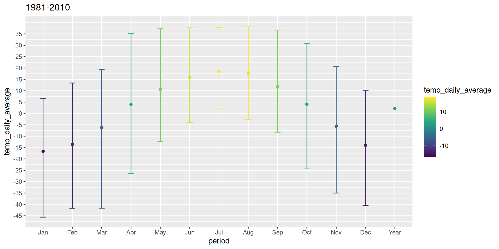
# rain_extreme_daily <dbl>, rain_extreme_daily_code <chr>, rain_extreme_daily_date <date>, …ggplot(data = normals, aes(x = period, colour = temp_daily_average)) +
geom_errorbar(aes(ymin = temp_extreme_min, ymax = temp_extreme_max), width = 0.2) +
geom_point(aes(y = temp_daily_average)) +
scale_colour_viridis_c() +
scale_y_continuous(breaks = seq(-50, 35, 5)) +
labs(title = normals$normals_years[1])Slides created with Quarto Updated 2025-10-27
There are no data for station 5256, in this time range (1950-07-01 to 1951-08-31), for this interval (day),
Available Station Data:
# A tibble: 2 × 17
  prov  station_name        station_id climate_id WMO_id TC_id   lat   lon  elev tz        interval start   end normals
  <chr> <chr>                    <dbl> <chr>       <dbl> <chr> <dbl> <dbl> <dbl> <chr>     <chr>    <dbl> <dbl> <lgl>
1 QC    ST ALEXIS DES MONTS       5256 7016816        NA <NA>   46.5 -73.2   183 Etc/GMT+5 day       1963  2025 TRUE
2 QC    ST ALEXIS DES MONTS       5256 7016816        NA <NA>   46.5 -73.2   183 Etc/GMT+5 month     1963  2018 TRUE
# ℹ 3 more variables: normals_1991_2020 <lgl>, normals_1981_2010 <lgl>, normals_1971_2000 <lgl># A tibble: 6 × 18
prov station_name station_id climate_id WMO_id TC_id lat lon elev tz interval start end normals
<chr> <chr> <dbl> <chr> <dbl> <chr> <dbl> <dbl> <dbl> <chr> <chr> <dbl> <dbl> <lgl>
1 QC ST ALEXIS DES MONTS 5256 7016816 NA <NA> 46.5 -73.2 183 Etc/G… day 1963 2025 TRUE
2 QC ST ALEXIS DES MONTS 5256 7016816 NA <NA> 46.5 -73.2 183 Etc/G… month 1963 2018 TRUE
3 QC ST PAULIN 5282 7017640 NA <NA> 46.4 -73.0 167 Etc/G… day 1950 1991 TRUE
4 QC ST PAULIN 5282 7017640 NA <NA> 46.4 -73.0 167 Etc/G… month 1951 1991 TRUE
5 QC ST CHARLES MANDEVILLE 2 5263 7016981 NA <NA> 46.4 -73.4 174. Etc/G… day 1968 1970 FALSE
6 QC ST CHARLES MANDEVILLE 2 5263 7016981 NA <NA> 46.4 -73.4 174. Etc/G… month 1968 1970 FALSE
# ℹ 4 more variables: normals_1991_2020 <lgl>, normals_1981_2010 <lgl>, normals_1971_2000 <lgl>, distance <dbl>library(mapview)
library(sf)
# Our point of interest
# lat, lon = 49.85, -99.91
# Get local stations
s <- stations_search(
coords = c(49.85, -99.91), interval = "day",
starts_latest = 2020,
ends_earliest = 2020) |> # lat, lon
st_as_sf(coords = c("lon", "lat"), crs = 4326)
p <- st_sfc(st_point(c(-99.91, 49.85)), crs = 4326) # lon, lat
# Interactive map of the stations with reference to our point of interest
mapview(s, zcol = "distance") + mapview(p, col.regions = "black", cex = 20)![]()