Special symbols in ggplot2

Creating ggplot2 figures with special characters such as superscripts (R²) math equations (\(\sqrt{x}\)) or greek letters (\(\omega\), \(\lambda\)), can be a bit of a headache.

I recently created some figures for my mom which required special characters in the axes as well as in annotations, and it reminded me of how much of a pain it can be, especially because depending on what you want to do, you need to use a different process for it.

If you want to create your annotations programatically (e.g., in a column of your data frame), you need a different process than if you were going to create them directly in the ggplot function calls.

There are also different layers in ggplots which require different inputs. Some can take an expression, and some only text, so you need to remember what to use for each of those.

So I decided to create this note as a reference for my future self, if for no one else 😁.

First we’ll go over when to use text vs. expressions and how to convert between the two for when you use them directly vs. programmatically. Then, because that’s super confusing, we’ll go through a bunch of examples of both.

Expression or text?

We’re going to be creating text with special symbols or characters by using plotmath and R expressions. For example, R^2 gives you \(R^2\). See ?plotmath or the Appendix table for how to code the symbols or expressions you want to use.

Sometimes ggplot needs this as text, sometimes as an expression.

Further, if you’re creating a label directly, it’s generally easier to create it as an expression and convert it to text if you need to.

On the other hand, if you’re creating labels programmatically, you’ll generally create them as text and will then have to convert to an expression as required.

In a nutshell…

For labels

• This includes name argument in scale_XXX() as well as labs()
• Direct Use: name = bquote(R^2)
• Programmatic Use: name = parse(text = "R^2")

For geoms

• This includes geom_text(), geom_label(), annotate(geom = "text") etc.
• Direct Use: label = deparse(bquote(R^2)), parse = TRUE¹
• Programmatic Use: label = "R^2", parse = TRUE
• parse = TRUE tells the function to turn the text into an expression

To summarize

Layer	Direct Use Create with expression	Programmatic Use Create with text
label requires expression	Expression bquote()	Parse text to expression parse(text = ""))
geom requires text	Deparse expression to text deparse(bquote()) and use parse = TRUE	Text ("") and use parse = TRUE

Expresssions

See ?plotmath or the Appendix table for how to code other symbols or expressions you want to use.

Here are some suggestions…

• Use “~” to create a space (or two!) between elements
• Use “*” to combine different elements without a space (think of this like a ‘,’ in R)
• Use quotes “” to mark normal text which has spaces and punctuation
• Use quotes, ~ and * around punctutation as needed (e.g., alpha*","~beta)
• Use == for equals (see Appendix table for more examples)
• Use ''^137*Cs when you need to put superscript before an element

bquote(R^2)  # Expression 

R^2

"R^2"        # Text

[1] "R^2"

You can test if you have created a text expression correctly by using parse(text = XXX)

parse(text = "R^2")

expression(R^2)

Example: Non-dynamic text (non-programmatic)

Here we create various non-dynamic text labels directly in the ggplot() code.

library(ggplot2)

ggplot() +
  theme_bw() +
  # Use `bquote()` in labels
  scale_x_continuous(name = bquote("Measurement"~(mu*g/L))) +
  scale_y_continuous(name = bquote(M/g)) +
  labs(title = bquote("Use quotes to mark normal text"~(mu*g/L)~(over(mu*g, L))~sqrt(x)),
       subtitle = bquote("Use ~ to link elements together with a space (or more!)"~~~~~alpha*","~beta*","~Gamma),
       caption = bquote(sum(x[i], i==1, n))) +
  # Use `deparse(bquote())` along with `parse = TRUE` in geoms
  annotate(geom = "text", x = 0.5, y = 0.5, label = deparse(bquote(P==0.001*";"~R^2==0.45)), parse = TRUE, size = 5) +
  geom_text(x = 0.5, y = 0.48, aes(label = deparse(bquote(''^137*Cs))), parse = TRUE, size = 5) +
  geom_text(x = 0.5, y = 0.52, aes(label = deparse(bquote(R[adj]^2==0.41))), parse = TRUE, size = 5)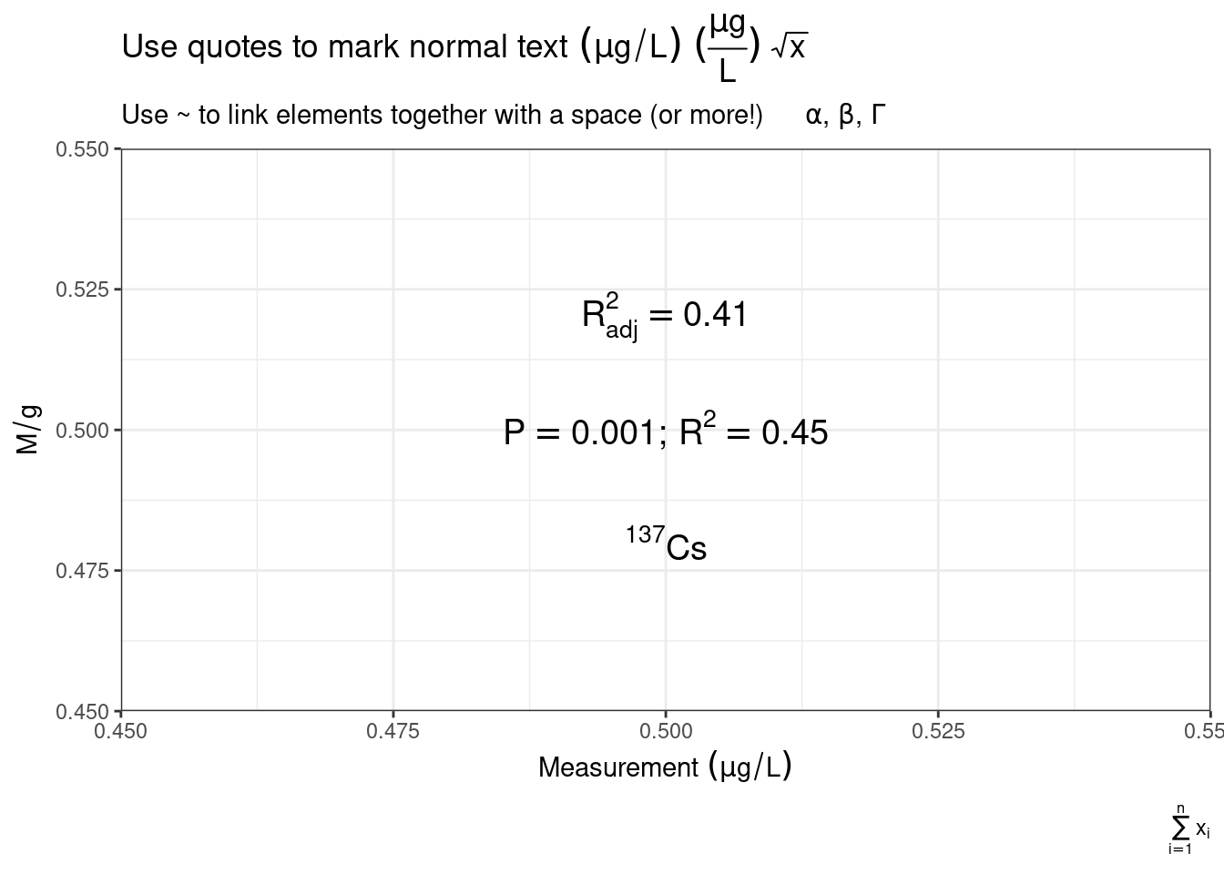

Example: Dynamic text (programmatic)

You’ll want to use dynamic or programmatic labels in situations where your labels are created in a data frame (e.g., different annotations for different facets in a plot, such as \(R^2\)s for different models, or special characters in your facet labels). Or perhaps you have a function which creates your plots.

First we’ll create some dynamic content to display. This will be text versions of plotmath expressions.

library(ggplot2)
library(palmerpenguins) # data
library(dplyr)  # manipulate the data

p <- mutate(penguins, sp = paste0("'", species, "'[(italic(", island, "))]"))

samples <- count(p, sp, species, island) |>
  mutate(label = paste0("n['(", species, ", ", island, ")'] == ", n))
samples

# A tibble: 5 × 5
  sp                            species   island        n label                 
  <chr>                         <fct>     <fct>     <int> <chr>                 
1 'Adelie'[(italic(Biscoe))]    Adelie    Biscoe       44 n['(Adelie, Biscoe)']…
2 'Adelie'[(italic(Dream))]     Adelie    Dream        56 n['(Adelie, Dream)'] …
3 'Adelie'[(italic(Torgersen))] Adelie    Torgersen    52 n['(Adelie, Torgersen…
4 'Chinstrap'[(italic(Dream))]  Chinstrap Dream        68 n['(Chinstrap, Dream)…
5 'Gentoo'[(italic(Biscoe))]    Gentoo    Biscoe      124 n['(Gentoo, Biscoe)']…

labels <- list("x" = paste0("'Bill Length'~mm[(", paste0(range(p$year), collapse = "-"), ")]"),
               "y" = paste0("'Flipper Length'~mm[(", paste0(range(p$year), collapse = "-"), ")]"))
labels

$x
[1] "'Bill Length'~mm[(2007-2009)]"

$y
[1] "'Flipper Length'~mm[(2007-2009)]"

Now let’s add this content to our plot

ggplot(data = p, aes(x = bill_length_mm, y = flipper_length_mm)) +
  geom_point() +
  geom_text(data = samples, x = -Inf, y = +Inf, aes(label = label), parse = TRUE,
            hjust = -0.1, vjust = 1.5) +
  facet_wrap(~ sp, labeller = label_parsed)

Warning: Removed 2 rows containing missing values or values outside the scale range
(`geom_point()`).

Example: Dynamic text - Advanced

As before, let’s start by creating some dynamic content to add to our plots. We’ll create this by creating text versions of the expressions we want to use.

• Note the use of {} around R^2 to ensure that the [adj] is actually subscript to the whole R^2, as opposed to just the the 2 (otherwise you’d get \(R^{2_{adj}}\)). Above, we just used a different order, R[adj]^2 to avoid this.
• Also note that the P-values are formatted to be either <=0.001 or format(nsmall = 3) to ensure there are always three digits after the decimal, and we then put the P-value in quotes (’’) because it is now text, not a number.

library(ggplot2)
library(palmerpenguins) # data
library(dplyr)  # manipulate the data
library(tidyr)  # unnest() to convert nested data back into a regular data frame
library(purrr)  # map() to loop over models and leables
library(broom)  # tidy() to extract model information

p <- penguins |>
  add_count(species) |>
  mutate(sp = paste0("'", species, "'"),
         sp = if_else(species == "Adelie", paste0(sp, "^{1}"), sp),
         sp = paste0(sp, "~(n == frac(", n, ", ", n(), "))"))

stats <- p |>
  nest(data = -"sp") |>
  mutate(model = map(data, \(x) lm(flipper_length_mm ~ bill_length_mm, data = x)),
         labels = map(model, glance)) |>
  unnest(cols = "labels") |>
  mutate(p_val = round(p.value, 3),
         p_val = if_else(p.value < 0.001, "<0.001", paste0("=='", format(p.value, nsmall = 3), "'")),
         stats = paste0("P", p_val, "*';'~{R^2}[adj]==", round(adj.r.squared, 2)))
select(stats, sp, stats)

# A tibble: 3 × 2
  sp                                 stats                       
  <chr>                              <chr>                       
1 'Adelie'^{1}~(n == frac(152, 344)) P<0.001*';'~{R^2}[adj]==0.1 
2 'Gentoo'~(n == frac(124, 344))     P<0.001*';'~{R^2}[adj]==0.43
3 'Chinstrap'~(n == frac(68, 344))   P<0.001*';'~{R^2}[adj]==0.21

labels <- list("x" = paste0("'Bill Length'~mm[(", paste0(range(p$year), collapse = "-"), ")]"),
               "y" = paste0("'Flipper Length'~mm[(", paste0(range(p$year), collapse = "-"), ")]"))
labels

$x
[1] "'Bill Length'~mm[(2007-2009)]"

$y
[1] "'Flipper Length'~mm[(2007-2009)]"

Now let’s add this to our plot

ggplot(data = p, aes(x = bill_length_mm, y = flipper_length_mm)) +
  geom_point() +
  geom_text(data = stats, x = -Inf, y = +Inf, aes(label = stats), parse = TRUE,
            hjust = -0.1, vjust = 1.5) +
  labs(x = parse(text = labels$x),
       y = parse(text = labels$y),
       caption = parse(text = "''^1*'Sampled on all three islands'")) +
  scale_y_continuous(limits = \(x) c(x[1], x[2]*1.04)) +
  facet_wrap(~ sp, labeller = label_parsed)

Warning: Removed 2 rows containing missing values or values outside the scale range
(`geom_point()`).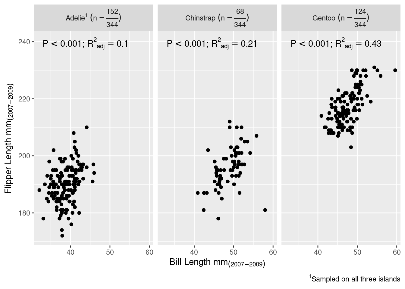

Troubleshooting

Errors

To find errors, test your labels with parse().

parse(text = "R^2")

expression(R^2)

parse(text = deparse(bquote(R^2)))

expression(R^2)

parse(text = p$sp[1])

expression("Adelie"^{
    1
} ~ (n == frac(152, 344)))

parse(text = labels$x)

expression("Bill Length" ~ mm[(2007 - 2009)])

parse(text = stats$stats[1])

expression(P < 0.001 * ";" ~ {
    R^2
}[adj] == 0.1)

You can also test them with bquote()

bquote(R^2)

R^2

If you have an error in your label, parse() (or bquote()) will fail.

parse(text = "R^^2")
bquote(R^^2)

Error: <text>:2:10: unexpected '^'
1: parse(text = "R^^2")
2: bquote(R^^
            ^

“unexpected string constant” OR “unexpected symbol”

• Did you remember to use * or ~ between separate elements?
• This is especially important between text elements

parse(text = "P==0.01';'R^2 == 0.45")

Error in parse(text = "P==0.01';'R^2 == 0.45"): <text>:1:8: unexpected string constant
1: P==0.01';'
           ^

parse(text = "P==0.01*';'~R^2==0.45")

expression(P == 0.01 * ";" ~ R^2 == 0.45)

Appendix: Plot math demos

If you run demo("plotmath"), you’ll get a series of tables showing the outputs of the plotmath codes in plots. However I don’t really like them, so here is my recreation using gt and ggplot2 (and some hacking of the documentation).

Note that there are some symbols that appear as white squares (especially lower in the table). This means that the font I’m using doesn’t support those symbols. If you get the same on a symbol you want to use, see about switching up your fonts. Unfortunately that is non-trivial 😢.

library(showtext)
library(stringr)
library(dplyr)
library(tidyr)
library(purrr)
library(ggplot2)
library(gt)

# Get the table
docs <- tools:::fetchRdDB(file.path(system.file("help", package = "grDevices"), "grDevices"))
docs <- docs$plotmath
docs <- capture.output(docs)
docs <- docs[-seq(1, str_which(docs, "\\\\tabular\\{ll\\}(?s).*"), 1)]
docs <- docs[-seq(str_which(docs, "^( )+\\}$")[1], length(docs), 1)]

# Extract the code and descriptions
labels <- docs |> 
  str_remove("\\\\cr") |>
  str_subset("Syntax", negate = TRUE) |>
  str_replace_all("\"", "'") |>
  str_squish() |>
  tibble(txt = _) |>
  filter(txt != "") |>
  separate("txt", into = c("code", "meaning"), sep = " \\\\tab ") |>
  mutate(code_raw = str_replace_all(code, "(\\\\code\\{)([^\\}]*)(\\})", "\\2"),
         code = paste0("`", code_raw, "`"),
         plot = 1:n(),
         code_raw = if_else(code_raw == "theta1, phi1, sigma1, omega1",
                            "theta1*phi1*sigma1*omega1", code_raw))

# Create a temp image of each symbol - image to that we get the correct
sysfonts::font_add(family = "dejavu", 
                   regular = "/usr/share/fonts/truetype/dejavu/DejaVuSans.ttf",
                   italic = "/usr/share/fonts/truetype/dejavu/DejaVuSans-Oblique.ttf",
                   bold = "/usr/share/fonts/truetype/dejavu/DejaVuSans-Bold.ttf",
                   bolditalic = "/usr/share/fonts/truetype/dejavu/DejaVuSans-BoldOblique.ttf"
                   )

g <- map2(labels$code_raw, labels$plot, \(x, i) {
  showtext_auto()
  ggplot() +
    theme_void() +
    geom_text(x = 0.5, y = 0.5, aes(label = x), parse = TRUE, size = 40, family = "dejavu")
})

# Create table of code plus symbol images
gt(labels) |>
  text_transform(locations = cells_body(columns = plot),
                 fn = function(x) ggplot_image(g[as.numeric(x)], height = px(50), aspect_ratio = 2)) |>
  cols_label(plot = "Plotted Symbol",
             code = "Code",
             meaning = "Description") |>
  cols_hide(code_raw) |>
  fmt_markdown(code)

Code	Description	Plotted Symbol
x + y	x plus y
x - y	x minus y
x*y	juxtapose x and y
x/y	x forwardslash y
x %+-% y	x plus or minus y
x %/% y	x divided by y
x %*% y	x times y
x %.% y	x cdot y
x[i]	x subscript i
x^2	x superscript 2
paste(x, y, z)	juxtapose x, y, and z
sqrt(x)	square root of x
sqrt(x, y)	yth root of x
x == y	x equals y
x != y	x is not equal to y
x < y	x is less than y
x <= y	x is less than or equal to y
x > y	x is greater than y
x >= y	x is greater than or equal to y
!x	not x
x %~~% y	x is approximately equal to y
x %=~% y	x and y are congruent
x %==% y	x is defined as y
x %prop% y	x is proportional to y
x %~% y	x is distributed as y
plain(x)	draw x in normal font
bold(x)	draw x in bold font
italic(x)	draw x in italic font
bolditalic(x)	draw x in bolditalic font
symbol(x)	draw x in symbol font
list(x, y, z)	comma-separated list
...	ellipsis (height varies)
cdots	ellipsis (vertically centred)
ldots	ellipsis (at baseline)
x %subset% y	x is a proper subset of y
x %subseteq% y	x is a subset of y
x %notsubset% y	x is not a subset of y
x %supset% y	x is a proper superset of y
x %supseteq% y	x is a superset of y
x %in% y	x is an element of y
x %notin% y	x is not an element of y
hat(x)	x with a circumflex
tilde(x)	x with a tilde
dot(x)	x with a dot
ring(x)	x with a ring
bar(xy)	xy with bar
widehat(xy)	xy with a wide circumflex
widetilde(xy)	xy with a wide tilde
x %<->% y	x double-arrow y
x %->% y	x right-arrow y
x %<-% y	x left-arrow y
x %up% y	x up-arrow y
x %down% y	x down-arrow y
x %<=>% y	x is equivalent to y
x %=>% y	x implies y
x %<=% y	y implies x
x %dblup% y	x double-up-arrow y
x %dbldown% y	x double-down-arrow y
alpha -- omega	Greek symbols
Alpha -- Omega	uppercase Greek symbols
theta1, phi1, sigma1, omega1	cursive Greek symbols
Upsilon1	capital upsilon with hook
aleph	first letter of Hebrew alphabet
infinity	infinity symbol
partialdiff	partial differential symbol
nabla	nabla, gradient symbol
32*degree	32 degrees
60*minute	60 minutes of angle
30*second	30 seconds of angle
displaystyle(x)	draw x in normal size (extra spacing)
textstyle(x)	draw x in normal size
scriptstyle(x)	draw x in small size
scriptscriptstyle(x)	draw x in very small size
underline(x)	draw x underlined
x ~~ y	put extra space between x and y
x + phantom(0) + y	leave gap for '0', but don't draw it
x + over(1, phantom(0))	leave vertical gap for '0' (don't draw)
frac(x, y)	x over y
over(x, y)	x over y
atop(x, y)	x over y (no horizontal bar)
sum(x[i], i==1, n)	sum x[i] for i equals 1 to n
prod(plain(P)(X==x), x)	product of P(X=x) for all values of x
integral(f(x)*dx, a, b)	definite integral of f(x) wrt x
union(A[i], i==1, n)	union of A[i] for i equals 1 to n
intersect(A[i], i==1, n)	intersection of A[i]
lim(f(x), x %->% 0)	limit of f(x) as x tends to 0
min(g(x), x > 0)	minimum of g(x) for x greater than 0
inf(S)	infimum of S
sup(S)	supremum of S
x^y + z	normal operator precedence
x^(y + z)	visible grouping of operands
x^{y + z}	invisible grouping of operands
group('(',list(a, b),']')	specify left and right delimiters
bgroup('(',atop(x,y),')')	use scalable delimiters
group(lceil, x, rceil)	special delimiters
group(lfloor, x, rfloor)	special delimiters
group(langle, list(x, y), rangle)	special delimiters

Resources

• ggplot2::geom_text()
• Stackoverflow question

Footnotes

1. You could also use straight text “R^2” without deparse(bquote()) if you wanted to work with text.