source("XX_functions.R") # Custom functions and packagesInitial Exploration
Background
This is the initial exploration of Turkey Vulture kettling and migration behaviour above Rocky Point on southern Vancouver Island.
Banding and observations start 1 hour before sunrise and commence for 6 hours. Blanks and ****** indicate no data (NA), often because the banding station was not open at all due to rainy weather or closed early for similar reasons. In addition, the station is on Department of National Defence land, and blanks can arise when banders are excluded by DND. Unfortunately, this applies to the entire year of 2007. Zero values represent true zeros, the count was made but no vultures seen.
Data values are daily estimates “of the greatest aggregation of vultures over Rocky Point that day during the station hours”.
Load & Clean Data
peek <- read_excel("Data/Raw/TUVU DET 1998-2023 days excluded FINAL_DLK_2025-05-28.xlsx")New names:
• `` -> `...1`
• `` -> `...28`
• `` -> `...29`
• `` -> `...30`
• `` -> `...31`
• `` -> `...32`
• `` -> `...33`
• `` -> `...34`
• `` -> `...35`end <- which(peek$`day/year` == "year") - 1
v <- read_excel("Data/Raw/TUVU DET 1998-2023 days excluded FINAL_DLK_2025-05-28.xlsx",
na = c("", "******"), n_max = end) New names:
• `` -> `...27`
• `` -> `...28`
• `` -> `...29`
• `` -> `...30`
• `` -> `...31`head(v)# A tibble: 6 × 31
`day/year` `1998` `1999` `2000` `2001` `2002` `2003` `2004` `2005`
<dttm> <dbl> <dbl> <dbl> <dbl> <dbl> <dbl> <dbl> <dbl>
1 2023-07-23 00:00:00 4 NA 2 4 3 4 3 3
2 2023-07-24 00:00:00 7 NA 0 3 4 5 3 4
3 2023-07-25 00:00:00 4 6 2 3 7 4 5 6
4 2023-07-26 00:00:00 0 4 0 2 6 5 4 6
5 2023-07-27 00:00:00 0 7 NA 9 5 1 1 1
6 2023-07-28 00:00:00 1 4 NA 10 7 6 1 8
# ℹ 22 more variables: `2006` <dbl>, `2008` <dbl>, `2009` <dbl>, `2010` <dbl>,
# `2011` <dbl>, `2012` <dbl>, `2013` <dbl>, `2014` <dbl>, `2015` <dbl>,
# `2016` <dbl>, `2017` <dbl>, `2018` <dbl>, `2019` <dbl>, `2020` <dbl>,
# `2021` <dbl>, `2022` <dbl>, `2023` <dbl>, ...27 <lgl>, ...28 <lgl>,
# ...29 <lgl>, ...30 <lgl>, ...31 <chr>tail(v)# A tibble: 6 × 31
`day/year` `1998` `1999` `2000` `2001` `2002` `2003` `2004` `2005`
<dttm> <dbl> <dbl> <dbl> <dbl> <dbl> <dbl> <dbl> <dbl>
1 2023-10-16 00:00:00 0 NA 0 NA 25 NA 120 5
2 2023-10-17 00:00:00 NA NA 4 NA 26 NA NA NA
3 2023-10-18 00:00:00 12 NA 4 NA 14 6 26 10
4 2023-10-19 00:00:00 NA 18 NA NA 8 NA NA NA
5 2023-10-20 00:00:00 NA 10 NA NA 17 NA NA NA
6 2023-10-21 00:00:00 NA NA NA NA 9 NA NA NA
# ℹ 22 more variables: `2006` <dbl>, `2008` <dbl>, `2009` <dbl>, `2010` <dbl>,
# `2011` <dbl>, `2012` <dbl>, `2013` <dbl>, `2014` <dbl>, `2015` <dbl>,
# `2016` <dbl>, `2017` <dbl>, `2018` <dbl>, `2019` <dbl>, `2020` <dbl>,
# `2021` <dbl>, `2022` <dbl>, `2023` <dbl>, ...27 <lgl>, ...28 <lgl>,
# ...29 <lgl>, ...30 <lgl>, ...31 <chr>v <- rename(v, date = "day/year") %>%
select(matches("date|\\d{4}")) %>%
assert(is.numeric, -"date") # make sure we get only numeric data, not summariesExpect 2023 for all years, as original data doesn’t include year and R must have a year (this is corrected below).
v# A tibble: 91 × 26
date `1998` `1999` `2000` `2001` `2002` `2003` `2004` `2005`
<dttm> <dbl> <dbl> <dbl> <dbl> <dbl> <dbl> <dbl> <dbl>
1 2023-07-23 00:00:00 4 NA 2 4 3 4 3 3
2 2023-07-24 00:00:00 7 NA 0 3 4 5 3 4
3 2023-07-25 00:00:00 4 6 2 3 7 4 5 6
4 2023-07-26 00:00:00 0 4 0 2 6 5 4 6
5 2023-07-27 00:00:00 0 7 NA 9 5 1 1 1
6 2023-07-28 00:00:00 1 4 NA 10 7 6 1 8
7 2023-07-29 00:00:00 0 5 0 2 6 1 3 1
8 2023-07-30 00:00:00 3 34 3 0 2 1 3 4
9 2023-07-31 00:00:00 4 11 4 8 2 7 2 3
10 2023-08-01 00:00:00 6 5 0 2 6 5 3 4
# ℹ 81 more rows
# ℹ 17 more variables: `2006` <dbl>, `2008` <dbl>, `2009` <dbl>, `2010` <dbl>,
# `2011` <dbl>, `2012` <dbl>, `2013` <dbl>, `2014` <dbl>, `2015` <dbl>,
# `2016` <dbl>, `2017` <dbl>, `2018` <dbl>, `2019` <dbl>, `2020` <dbl>,
# `2021` <dbl>, `2022` <dbl>, `2023` <dbl>v <- v |>
mutate(`2007` = NA) |> # Add missing year for completeness
relocate("2007", .before = "2008") |>
pivot_longer(-date, names_to = "year", values_to = "count")
year(v$date) <- as.integer(v$year) # Fix years for each date
v <- mutate(v, date = as_date(date), doy = yday(date))Correct year on all dates now, and verify a couple of random dates.
v %>%
  verify(is.na(count[date == "1999-07-23"])) %>%
  verify(count[date == "2006-08-06"] == 7) %>%
  verify(count[date == "2020-09-26"] == 50) %>%
  verify(count[date == "2023-10-14"] == 54)
# A tibble: 2,366 × 4
date year count doy
<date> <chr> <dbl> <dbl>
1 1998-07-23 1998 4 204
2 1999-07-23 1999 NA 204
3 2000-07-23 2000 2 205
4 2001-07-23 2001 4 204
5 2002-07-23 2002 3 204
6 2003-07-23 2003 4 204
7 2004-07-23 2004 3 205
8 2005-07-23 2005 3 204
9 2006-07-23 2006 4 204
10 2007-07-23 2007 NA 204
# ℹ 2,356 more rowsQuick look at the data
Too see full screen: Right-click and select “Open Image in New Tab” (or similar)
ggplot(v, aes(x = doy, y = count, group = year, colour = year)) +
  theme_bw() +
  geom_point(na.rm = TRUE) +
  stat_smooth(method = "gam", formula = y ~ s(x, k = 20),
              method.args = list(method = "REML", family = "nb"), na.rm = TRUE,
              level = 0.95) +
  facet_wrap(~year, scales = "free") +
  scale_colour_viridis_d()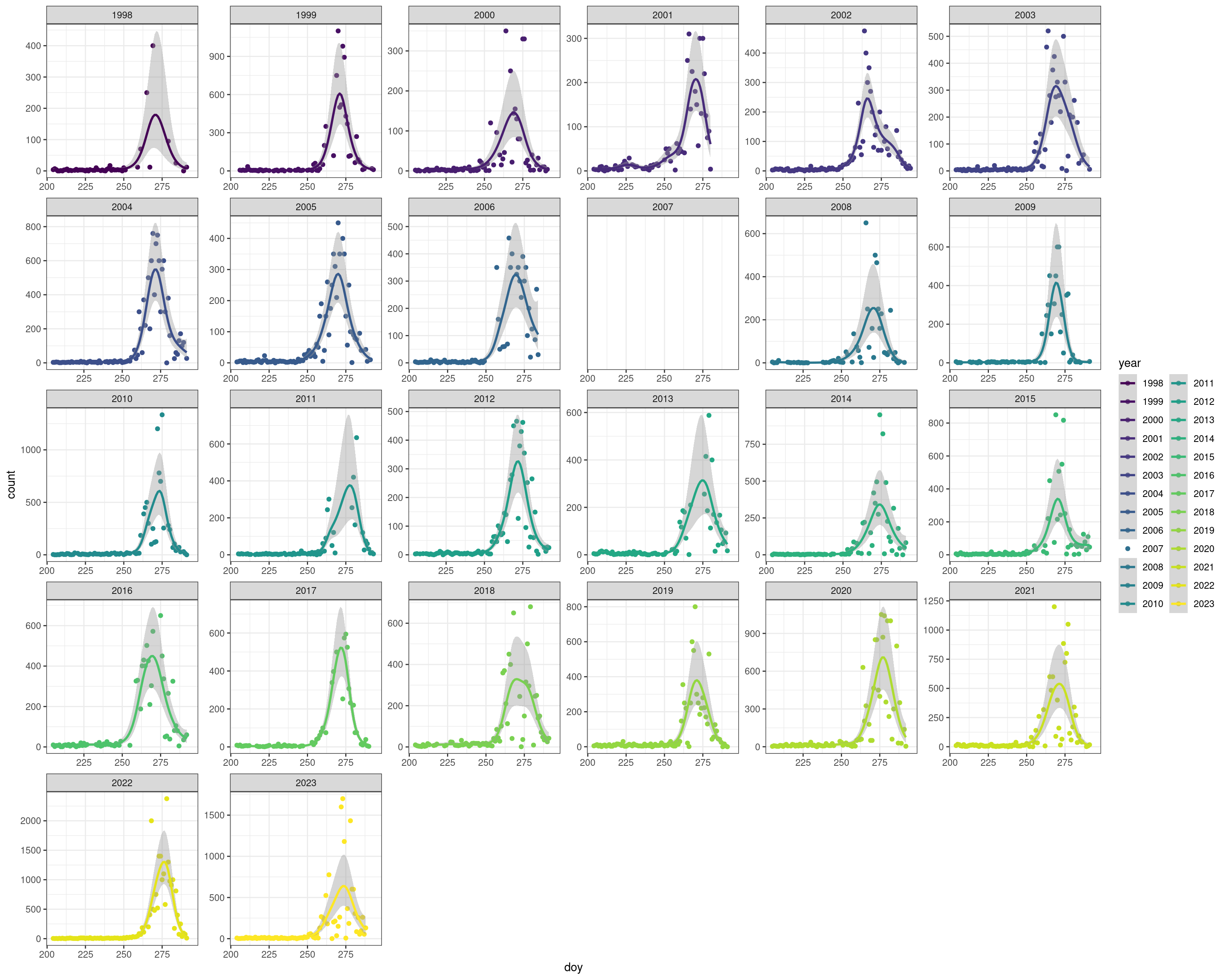
Omit 1998 because missing almost all of the second half of the migration period.
v <- filter(v, year != 1998)Save this formatted data for later use
write_csv(v, "Data/Datasets/vultures_clean_2023.csv")Questions
- Has the timing of kettle formation and migration has changed over the years?
- If so, what is the pattern of change? (Direction and magnitude of change)
- If not, document temporal distribution of numbers
- Has the number of birds in the kettles changed over time?
- may indicate population trends
- complicated by accumulating birds over days when the weather conditions are not suitable for passing over the strait
- potentially look at weather effects…
Metrics to assess
To answer these questions we need to summarize the counts into specific metrics representing the timing of migration.
Specifically, we would like to calculate the
- dates of 5%, 25%, 50%, 75%, and 95% of the kettle numbers
- duration of passage - No. days between 5% and 95%
- duration of peak passage - No. days between 25% and 75%
Population size (no. vultures in aggregations)
- maximum
- cumulative
- number at peak passage (max? range? median?)
- mean/median number of locals
Of these, the most important starting metrics are the dates of 5%, 25%, 50%, 75%, and 95% of the kettle numbers. These dates will define migration phenology as well as local vs. migrating counts. All other calculations can be performed using these values and the raw data.
How to calculate dates of passage?
- Don suggested following methodology from Allcock et al 2022
- “fit a curve to the data for each year and use it to estimate …”
- Allcock et al 2022 “modelled optimal Gaussian functions to describe the migration phenology for each species – year combination in our dataset using Markhov Chain Monte Carlo (MCMC) techniques”.
- They say that “Gaussian functions … often outperform General Additive Models (Linden et al., 2016)”
I like this approach in general, but I’m not convinced that we can’t/shouldn’t use GAMs.
In Linden et al., they restricted the GAM models’ effective degrees of freedom (which isn’t common, usually they are determined by the modelling procedure) and note that if they didn’t restrict them, “GAMs would have been preferred in 73% of the cases”.
The argument for restricting GAMS was to make the comparison among models possible as the “estimation of [effective] degrees of freedom [in a GAM] is similar to a model selection procedure”. This would have invalidated their use of the information theoretic approach for model comparison.
I still think we should use GAMs, because
- We are using this to calculate metrics and as long as the model fits the data, is consistent and replicable, it doesn’t really matter how we get there (i.e. there’s no reason to not use the best GAM method with built-in model selection).
- We are looking at a single species and so can assess each year to make sure it looks right.
- I am familiar with GAMs, but have no experience with MCMC techniques to model Gaussian functions.
- I don’t think that Linden et al. really demonstrated that GAMs are ‘bad’ to use.
Steffi’s suggested approach
We use GAMs to model each year individually. From the predicted data we calculate the cumulative counts and the points at which these counts hit 5%, 25%, 75%, 95% of the total (I think this is what Allcock et al mean by ‘bird-days’?).
However, we will need to think about how to handle the resident birds, as they may artificially inflate the cumulative counts prior to migration.
Using GAM based appraoch
For illustration and exploration of this approach, we’ll look at 2000.
- Negative binomial model fits the count data with overdispersion
- Use Restricted Maximum Likelihood (“Most likely to give you reliable, stable results”1)
- We smooth (
s()) overdoy(day of year) to account for non-linear migration patterns - We set
k = 10(up to 10 basis functions; we want enough to make sure we capture the patterns, but too many will slow things down).
g <- gam(count ~ s(doy, k = 10), data = filter(v, year == 2000),
         method = "REML", family = "nb")
plot(g, shade = TRUE, trans = exp, residuals = TRUE, pch = 20,
     shift = coef(g)[1])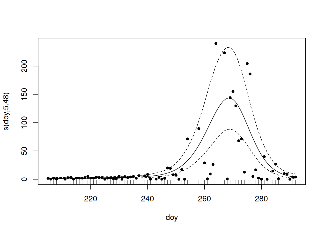
Not really necessary for us to evaluate, but the s(doy) value indicates that we have a signifcant pattern, and the fact that the edf value is less than our k = 10, is good.
summary(g)
Family: Negative Binomial(1.129)
Link function: log

Formula:
count ~ s(doy, k = 10)

Parametric coefficients:
            Estimate Std. Error z value Pr(>|z|)
(Intercept)   2.3393     0.1207   19.38   <2e-16 ***
---
Signif. codes:  0 '***' 0.001 '**' 0.01 '*' 0.05 '.' 0.1 ' ' 1

Approximate significance of smooth terms:
         edf Ref.df Chi.sq p-value
s(doy) 5.475  6.616  175.5  <2e-16 ***
---
Signif. codes:  0 '***' 0.001 '**' 0.01 '*' 0.05 '.' 0.1 ' ' 1

R-sq.(adj) =  0.391   Deviance explained = 71.3%
-REML =  271.2  Scale est. = 1         n = 76
Quick checks to ensure model is valid.
Code
p0 <- par(mfrow = c(2,2))
gam.check(g, pch = 19, cex = 0.5)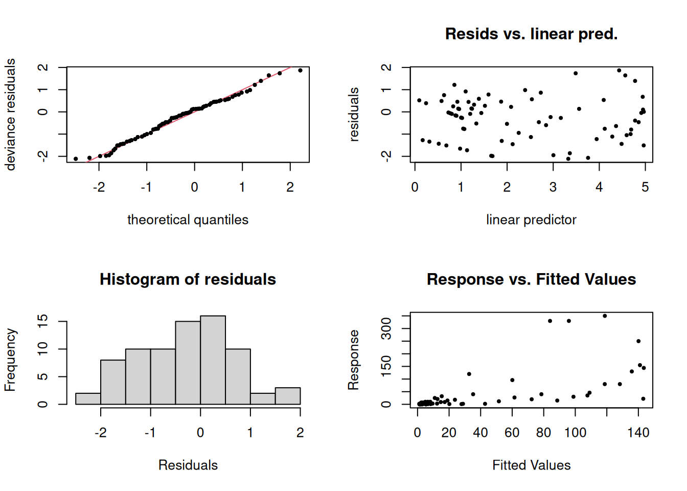
Method: REML   Optimizer: outer newton
full convergence after 4 iterations.
Gradient range [8.674563e-10,1.084888e-07]
(score 271.1993 & scale 1).
Hessian positive definite, eigenvalue range [2.264941,28.62155].
Model rank =  10 / 10

Basis dimension (k) checking results. Low p-value (k-index<1) may
indicate that k is too low, especially if edf is close to k'.

         k'  edf k-index p-value
s(doy) 9.00 5.48    0.96    0.62
Code
par(p0)

s <- DHARMa::simulateResiduals(g, plot = TRUE)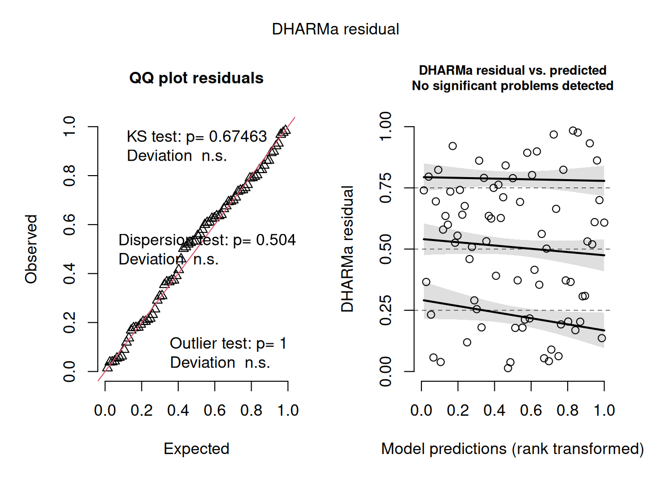
Calculating dates of passage
First create data set of predicted GAM model outputs across the entire date range.
doy <- min(g$model$doy):max(g$model$doy)

p <- predict(g, newdata = list(doy = doy), type = "response", se.fit = TRUE)
d <- data.frame(doy = doy, count = p$fit, se = p$se) |>
  mutate(ci99_upper = count + se * 2.58,
         ci99_lower = count - se * 2.58)
Next we’ll calculate percentiles based on cumulative counts. But there are several ways we can do this, depending how we want to account for resident vultures.
- Option 1: We do nothing
- Option 2: We use the model’s CI 99% to find a threshold date before which we assume all observations are of local, resident vultures, after which is migration. We would then calculate cumulative counts only on data after this threshold)2
- Option 3: We calculate the median number of residents and simply subtract that from all counts before calculating our cumulative counts.
Option 1: Do not omit resident vultures
- Use entire date range
- No threshold cutoff
- No subtraction of local counts
- Calculate local counts from predicted data before Day 240
Code
d_sum <- mutate(d, count_sum = cumsum(count))

dts <- calc_dates(d_sum)
dts_overall <- mutate(dts, type = "Option 1: No Adjustments")

residents <- d |>
  filter(doy < 240) |>
  summarize(res_pop_min = min(count), res_pop_max = max(count),
            res_pop_median = median(count), res_pop_mean = mean(count)) |>
  mutate(across(everything(), \(x) round(x, 1)))

g1 <- plot_cum_explore(d_sum = d_sum, dts = dts)
g2 <- plot_model_explore(d_raw = g$model, d_pred = d, dts = dts, residents, resident_date = 240) +
  labs(caption = "Local count stats calculated up to Day 240")
g_opt1 <- g1 / g2 + plot_annotation(title = "Option 1: No adjustments")
Option 2: Use a count threshold to omit dates with resident vultures
- Use the minimum value of the upper limit of the CI 99% to calculate a cutoff threshold (only consider dates < 270 to avoid the end of migration tailing off)
- The first date prior to migration which crosses this threshold into migration (i.e. avoids little blips up and down early in the year) is used as the threshold
- The data is filtered to include only dates on or after this threshold
- Then the percentiles are calculated based on cumulative counts in this subset
thresh <- filter(d, doy < 270) |> # Only consider pre-migration
  arrange(desc(doy)) |>
  filter(count <= min(ci99_upper)) |>
  slice(1) |>
  pull(doy)
thresh
[1] 228What is the min of the upper limit of the CI 99%?!?!?
In the image below…
- the Grey ribbon represents the 99% Confidence Interval around the GAM model (grey line)
- the upper limit of this ribbon is the upper limit of the 99% CI
- the minimum of this value is the area on the figure where the upper edge of the ribbon is at it’s lowest value (large black point)
- in this year/model, it’s occurs on the first day
How do we use this value?
- the first value in the model (grey line) to cross this limit (dashed black line), identifies our threshold date (red dashed line)
- we then use only the dates after this threshold to calculate migration metrics
- we then use only the dates before this threshold to calculate local counts
Code
# g1 <- ggplot(data = d, mapping = aes(x = doy, y = count)) +
#   theme_bw() +
#   geom_ribbon(aes(ymin = ci99_lower, ymax = ci99_upper), fill = "grey50", alpha = 0.5) +
#   geom_point(data = g$model) +
#   geom_line() +
#   coord_cartesian(xlim = c(204, 270)) +
#   labs(title = "Look only at beginning of migration")

g2 <- ggplot(data = d, mapping = aes(x = doy, y = count)) +
  theme_bw() +
  theme(legend.position = c(0.3, 0.85), legend.title = element_blank()) +
  geom_ribbon(aes(ymin = ci99_lower, ymax = ci99_upper), fill = "grey50", alpha = 0.3) +
  geom_point(data = g$model, colour = "grey40") +
  geom_line(colour = "grey60") +
  coord_cartesian(xlim = c(204, 245), ylim = c(-5, 40)) +
  geom_point(x = d$doy[d$ci99_upper == min(d$ci99_upper)],
             y = min(d$ci99_upper), size = 4, aes(colour = "Day with min 99% CI"),
             inherit.aes = FALSE) +
  geom_hline(linetype = 2,
             aes(yintercept = min(d$ci99_upper), colour = "Min of upper 99% CI")) +
  geom_vline(linetype = 2,
             aes(xintercept = thresh, colour = "Threshold\n(first date consistently\nabove min of upper 99% CI)")) +
  scale_colour_manual(values = c("black", "black", "red")) +
  guides(colour = guide_legend(override.aes = list(shape = c(19, 0, 0), size = c(3, 0, 0), linewidth = c(0, 0.3, 0.3), linetype = c("solid", "dashed", "dashed")))) +
  labs(title = "Find thresholds based on local counts",
       subtitle = "Figure is model plot 'zoomed' into early season")
Warning: A numeric `legend.position` argument in `theme()` was deprecated in ggplot2
3.5.0.
ℹ Please use the `legend.position.inside` argument of `theme()` instead.Code
g2Warning in geom_point(x = d$doy[d$ci99_upper == min(d$ci99_upper)], y = min(d$ci99_upper), : All aesthetics have length 1, but the data has 88 rows.
ℹ Please consider using `annotate()` or provide this layer with data containing
a single row.Warning: Use of `d$ci99_upper` is discouraged.
ℹ Use `ci99_upper` instead.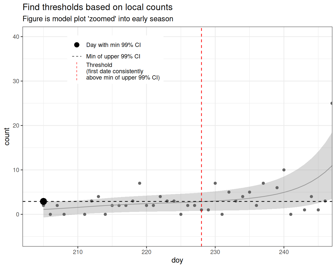
Code
d_sum <- filter(d, doy >= thresh) |>
  mutate(count_sum = cumsum(count))

dts <- calc_dates(d_sum)
dts_overall <- bind_rows(dts_overall,
                         mutate(dts, type = "Option 2: Threshold"))

residents <- d |>
  filter(doy < thresh) |>
  summarize(res_pop_min = min(count), res_pop_max = max(count),
            res_pop_median = median(count), res_pop_mean = mean(count)) |>
  mutate(across(everything(), \(x) round(x, 1)))


g1 <- plot_cum_explore(d_sum, dts) +
  geom_vline(xintercept = thresh, colour = "red", linetype = "dotted") +
  annotate("text", label = "Threshold", x = thresh, y = 1000)
g2 <- plot_model_explore(d_raw = g$model, d_pred = d, dts = dts, residents, resident_date = thresh) +
  labs(caption = paste0("Resident count stats calculated up to threshold date, ", thresh))

g_opt2 <- g1 / g2 + plot_annotation(title = "Option 2: Use only dates after threshold")
Option 3: Subtract the median resident count from all observations
- Use entire date range
- No threshold cutoff
- Subtract the median resident count from the predicted observations, prior to calculating the cumulative counts
- Calculate resident counts from predicted data before Day 240
Code
residents <- d |>
  filter(doy < 240) |>
  summarize(res_pop_min = min(count), res_pop_max = max(count),
            res_pop_median = median(count), res_pop_mean = mean(count)) |>
  mutate(across(everything(), \(x) round(x, 1)))

d_sum <- mutate(d,
                count = count - residents$res_pop_median,
                count_sum = cumsum(count))

dts <- calc_dates(d_sum)
dts_overall <- bind_rows(dts_overall,
                         mutate(dts, type = "Option 3: Subtraction"))

g1 <- plot_cum_explore(d_sum = d_sum, dts = dts) +
  annotate("text", x = 225, y = 1000,
           label = paste0("Remove ",
                          residents$res_pop_median,
                          " from all counts\nbefore calcuating cumuative sum"))
g2 <- plot_model_explore(d_raw = g$model, d_pred = d, dts = dts, residents, resident_date = 240) +
  labs(caption = "Local count stats calculated up to Day 240")
g_opt3 <- g1 / g2 + plot_annotation(title = "Option 3: Subtract median first")
Comparing our options
In each figure the red dots represent the 5%, 25%, 50%, 75% and 95% dates calculated based on the cumulative counts (top figure, dotted lines show the percentiles).
The bottom figure shows the raw counts, with the GAM model overlaid, the pink windows indicate 5%-95% and 25%-75% date ranges. The arrow on the left indicates which predicted values were included in the local count statistics.
Note that the only two things that really change in this example are the initial 5% date (becomes increasingly later with each option) and the calculation of the “local” population statistics (because in Option 1 and Option 2, they’re based on the same set of data, but in Option 2, we use a threshold to define before and after the expected start of migration.
g_opt1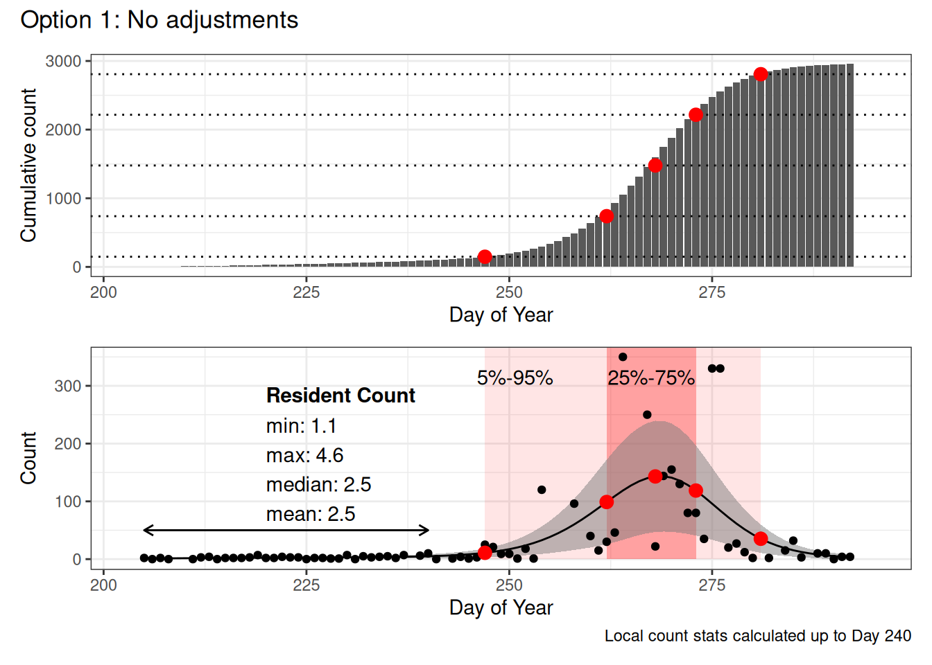
g_opt2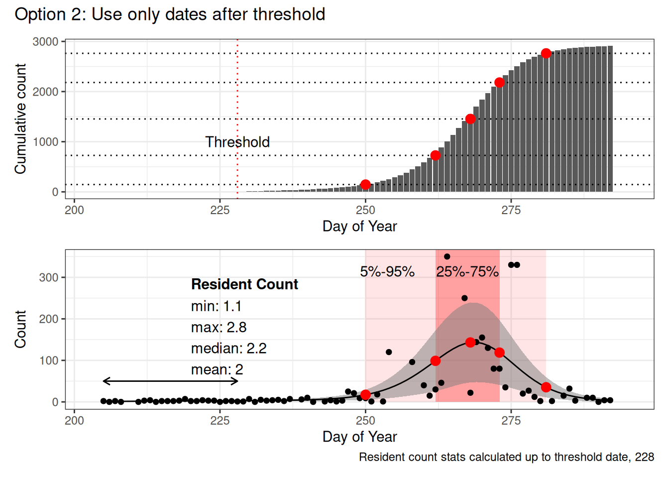
g_opt3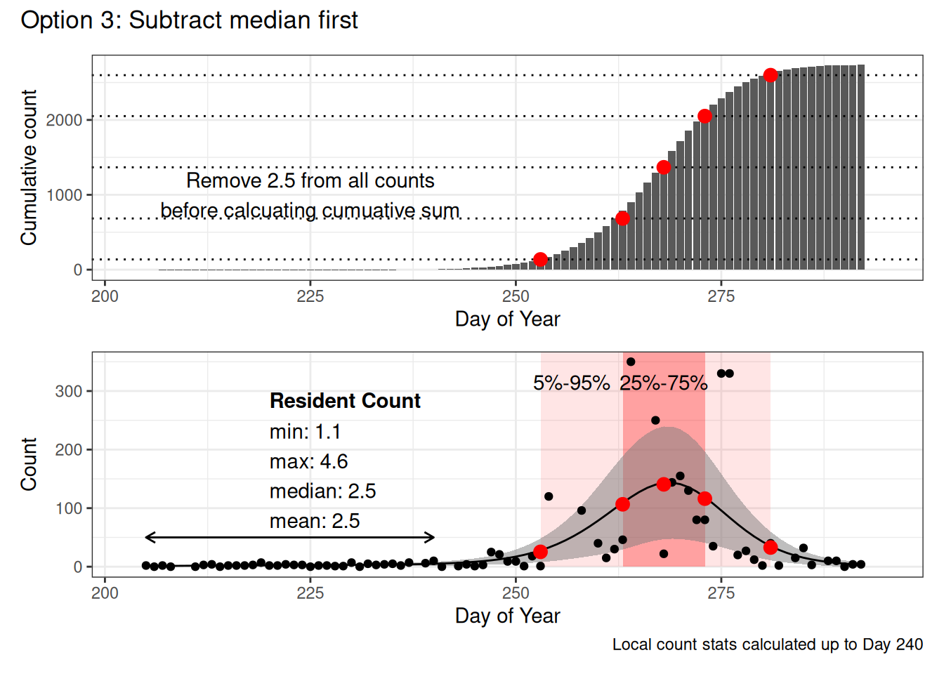
However in this example (and in many that I’ve looked at), this only really affects the first, 5%, Date value.
Here are the dates calculated for each percentiles using the different methods in this example.
dts_overall |>
  select(-contains("count")) |>
  pivot_wider(names_from = "perc", values_from = "doy_passage")
# A tibble: 3 × 6
type p05 p25 p50 p75 p95
<chr> <dbl> <dbl> <dbl> <dbl> <dbl>
1 Option 1: No Adjustments 247 262 268 273 281
2 Option 2: Threshold 250 262 268 273 281
3 Option 3: Subtraction 253 263 268 273 281Steffi’s suggested approach
I suggest we use Option 3: Subtracting the median local numbers.
I think that Option 1 gives us an artifically early start to migration as it starts cumulating counts over resident bird observations.
I think that Option 2 works, but is potentially overly complicated. I’m also not convinced that it completely avoids the issue of resident birds.
On the other hand I find Option 3
- Reasonable
- Easy to explain
- Visually, it looks the most ‘right’ (to me at any rate)
- It seems to result in more conservative numbers
Other options
- We could also just not use the 5% and 95% metrics
- I could run all three methods on the full data set and we could check them all together.
Reproducibility
Footnotes
https://noamross.github.io/gams-in-r-course/chapter1↩︎
Similar to a method I used in a paper with Matt Reudink on Bluebirds and also one on Swifts (companion to the one you referenced). We used this to calculate a threshold for latitude to define the start and end of migration by population postition rather than counts, though.↩︎