Manuscript Figure and Supplemental

This is the final figure and Supplemental material for the manuscript.

Setup

source("XX_functions.R")  # Custom functions and packages

# Metrics
v <- read_csv("Data/Datasets/vultures_final.csv") |>
  # Round non-integer values of population counts
  mutate(across(c(contains("pop"), contains("raw")), round)) 

# Raw counts
raw <- read_csv("Data/Datasets/vultures_clean_2023.csv")

# Predicted GAM models
pred <- read_csv("Data/Datasets/vultures_gams_pred.csv")

# Checking problematic years
supp <- read_csv("Data/Datasets/table_supplemental.csv")

Main figure

v <- v |> 
  mutate(date = as_date(p50_doy) - days(1))

g1 <- ggplot(v, aes(x = year, y = date)) +
  theme_bw() +
  theme(axis.title.x = element_blank()) +
  geom_point() +
  geom_smooth(method = "lm", se = TRUE) +
  labs(y = "Date of peak migration", x = "")

g2 <- ggplot(v, aes(x = year, y = mig_raw_max)) +
  theme_bw() +
  geom_point() +
  stat_smooth(method = MASS::glm.nb) +
  labs(y = "Annual maximum\nDaily Estimated Total", x = "Year")

g <- g1 / g2 + plot_annotation(tag_levels = "A")
#ggsave("fig1_quick.png", dpi = 1000, width = 8, height = 7)

gg <- g1 / (g2 + labs(y = "Annual maximum DET")) + plot_annotation(tag_levels = "A")

Double checking growth and increases

m <- MASS::glm.nb(mig_raw_max ~ year, data = v)

d <- select(v, year) |>
  mutate(y = predict(m, v),
         yexp = exp(y))

# Compound growth (avg growth over the period)
(1251 / 451)^ (1/25) - 1

[1] 0.04165339

# Compound interest (amount at the end)
451 * (1 + 0.041647)^(25)

[1] 1250.808

# Factor of increase
1251/451

[1] 2.773836

Big version

With two y-axis options for panel B

g

`geom_smooth()` using formula = 'y ~ x'
`geom_smooth()` using formula = 'y ~ x'

gg

`geom_smooth()` using formula = 'y ~ x'
`geom_smooth()` using formula = 'y ~ x'

Small version

With two y-axis options for panel B

g

`geom_smooth()` using formula = 'y ~ x'
`geom_smooth()` using formula = 'y ~ x'

gg

`geom_smooth()` using formula = 'y ~ x'
`geom_smooth()` using formula = 'y ~ x'

Map

library(bcmaps)

Support for Spatial objects (`sp`) was removed in {bcmaps} v2.0.0. Please use `sf` objects with {bcmaps}.

library(ggrepel)
ne_download(type = "populated_places", scale = "large", load = FALSE)

[1] "ne_10m_populated_places"

cities <- bcmaps::bc_cities(ask = FALSE) |> 
  select(NAME) |>
  filter(NAME %in% c("Victoria", "Vancouver", "Nanaimo"))

bc_cities was updated on 2024-07-10

cities <- ne_load(file_name = "ne_10m_populated_places") |> 
  filter(NAME %in% c("Seattle", "Portland"), ADM1NAME %in% c("Oregon", "Washington")) |>
  select(NAME) |> 
  st_transform(st_crs(cities)) |>
  bind_rows(cities) |>
  rename(name = NAME)

Reading layer `ne_10m_populated_places' from data source 
  `/home/steffi/R_tmpdir/Rtmp1ic9bU/ne_10m_populated_places.shp' 
  using driver `ESRI Shapefile'
Simple feature collection with 7342 features and 137 fields
Geometry type: POINT
Dimension:     XY
Bounding box:  xmin: -179.59 ymin: -90 xmax: 179.3833 ymax: 82.48332
Geodetic CRS:  WGS 84

stn <- c(-123.55082035835214, 48.31773308537152) |>
  st_point() |>
  st_sfc(crs = 4326) |>
  st_sf(name = "Rocky Point") |>
  st_transform(st_crs(cities))

land <- data.frame(lon = c(-124.3, -124.3, -123.5),
                   lat = c(48.39, 48.75, 49.2),
                   name = c("Juan de Fuca Strait", "Vancouver Island", "Salish Sea")) |>
  st_as_sf(coords = c("lon", "lat"), crs = 4326)

area <- ne_states(country = c("Canada", "United States of America")) |>
  #st_crop(st_bbox(c(xmin = -140, xmax = -112, ymin = 41, ymax = 60))) |>
  #filter(name %in% c("British Columbia", "Alberta", "Washington", "Oregon", "Idaho", "Montana")) |>
  mutate(
    name = if_else(name %in% c("British Columbia", "Washington", "Oregon"), toupper(name), NA),
    name = str_replace(name, " ", "\n"),
    postal =  if_else(postal %in% c("BC", "WA", "OR", "AB"), postal, NA))

box <- st_polygon(list(rbind(c(1050000, 330000), 
                             c(1050000, 490000),
                             c(1230000, 490000),
                             c(1230000, 330000),
                             c(1050000, 330000)))) |>
  st_sfc(crs = 3005)

g0 <- ggplot(data = area, aes(label = name)) +
  theme_map() +
  theme(panel.border = element_rect(fill = NA), 
        plot.margin = unit(c(0,0,0,0), units = "mm"),
        panel.spacing = unit(0, units = "mm")) +
  scale_x_continuous(expand = c(0,0)) +
  scale_y_continuous(expand = c(0,0)) +
  geom_sf()
  
g <- g0 +
  geom_sf(data = stn, size = 3) +
  geom_sf_text(data = stn, lineheight = 0.85, nudge_y = -8000) +
  geom_sf(data = cities) +
  geom_sf_text(data = cities, hjust = 1.1, nudge_y = 5000) +
  geom_sf_text(data = land, angle = c(-24, 0, -45), colour = "grey60", size = c(6, 7, 7)) +
  annotation_scale(location = "bl") + 
  annotation_north_arrow(
    location = "bl", height = unit(0.5, "cm"), width = unit(0.5, "cm"),
    style = north_arrow_orienteering(text_size = -Inf), pad_y = unit(0.75, "cm")) +
  coord_sf(crs = 3005, xlim = c(1050000, 1230000), ylim = c(330000, 490000))

g_inset <- g0 +
  theme(panel.background = element_rect(fill = "white")) +
  geom_sf_text(aes(label = postal), colour = "black", size = 3) +
  geom_sf(data = box, fill = NA, linewidth = 0.5, colour = "black", inherit.aes = FALSE) +
  coord_sf(crs = 3005, xlim = c(500000, 2000000), ylim = c(-200000, 1370000))

Big

g + inset_element(g_inset, left = 0, top = 1, bottom = 0.6, right = 0.342, align_to = "full")

Warning: Removed 60 rows containing missing values or values outside the scale range
(`geom_text()`).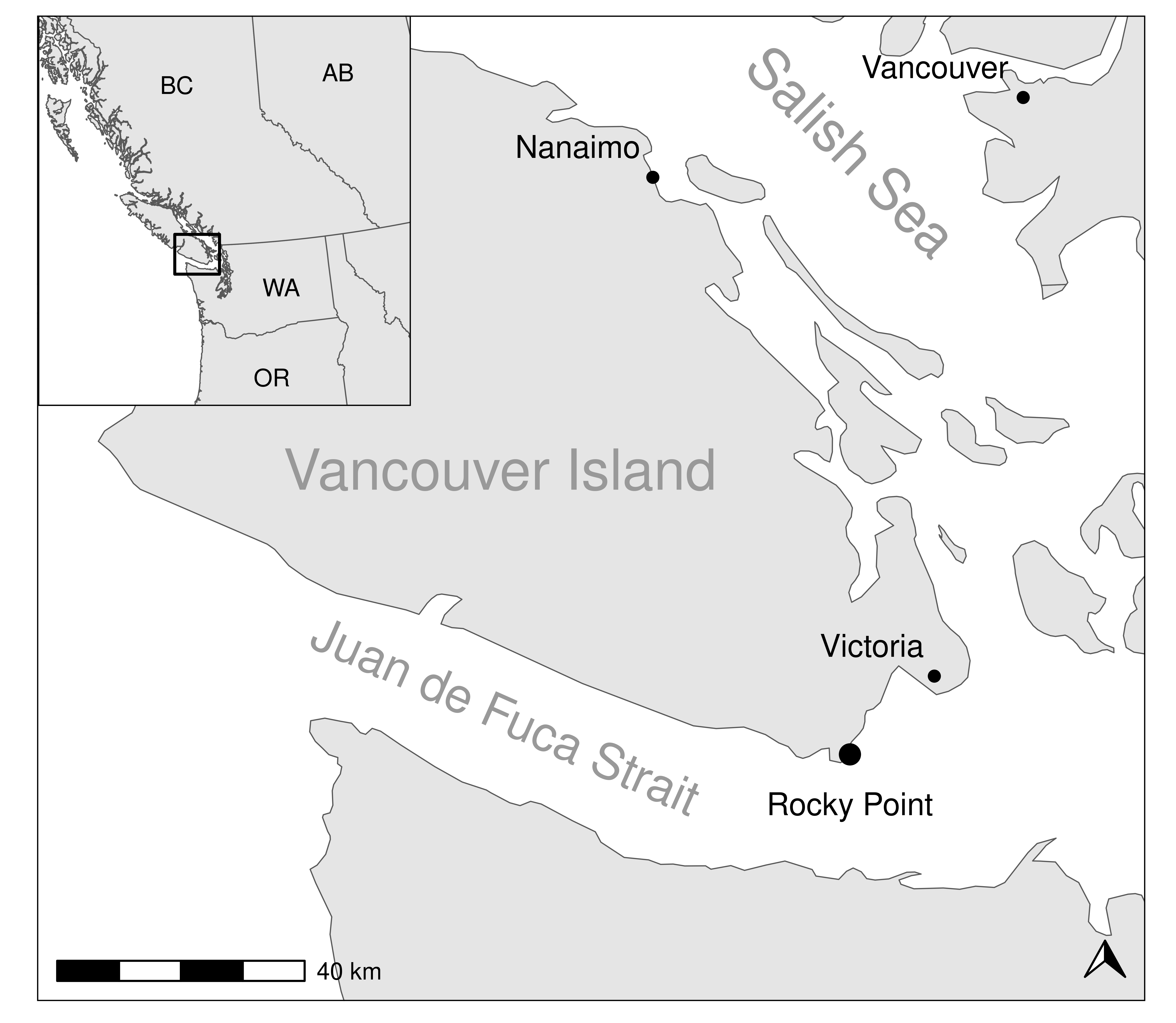

Small

g + inset_element(g_inset, left = 0, top = 1, bottom = 0.6, right = 0.342, align_to = "full")

Warning: Removed 60 rows containing missing values or values outside the scale range
(`geom_text()`).

Supplemental Figure

pred <- mutate(pred, ci95_upper = count + se * 1.96, ci95_lower = count - se * 1.96)
res <- filter(v, year == 1999) |>
  mutate(xmin = 204, 
         xmax = 240, y = 0.25 * mig_raw_max, 
         xmid = (240-204)/2 + 204,
         y = 0.25 * mig_raw_max,
         height = 0.03 * mig_raw_max, label = "Resident period")

g0 <- ggplot() +
  theme_void() +
  annotate(geom = "text", label = c("Migration\nstart", "Peak\nstart", "Peak", "Peak\nend", "Migration\nend"), 
           y = -0.25, x = c(0, 0.7, 1.3, 1.6, 2), size = 3, lineheight = 0.85) +
  annotate(geom = "text", label = c("5%", "25%", "50%", "75%", "95%"), y = 0.25, x = c(0, 0.7, 1.3, 1.6, 2), size = 3) +
  annotate(geom = "segment", y = 0, x = 0, xend = 2, arrow = arrow(angle = 90, ends = "both", length = unit(1, "mm"))) +
  annotate(geom = "segment", y = 0, x = 0.7, xend = 1.6, linewidth = 4) +
  annotate(geom = "segment", x = 1.29, xend = 1.30, y = 0, linewidth = 8) +
  ylim(c(-0.5, 0.5)) +
  xlim(c(-0.1, 2.1))

g1 <- ggplot(data = pred, mapping = aes(x = doy, y = count)) +
  theme_bw() +
  
  # GAM
  geom_ribbon(aes(ymin = ci95_lower, ymax = ci95_upper), fill = "grey50", alpha = 0.5) +
  geom_line() +
  
  # Raw points
  geom_point(data = raw, na.rm = TRUE, size = 0.5) +
  
  # Metrics
  geom_errorbarh(data = res, aes(xmin = xmin, xmax = xmax, y = y, height = height), 
                 colour = "grey70", inherit.aes = FALSE) +
  geom_text(data = res, aes(x = xmid, y = y, label = label), vjust = -0.5, inherit.aes = FALSE,
            size = 3, colour = "grey30") +
  geom_segment(data = v, aes(x = p50_doy - 0.5, xend = p50_doy + 0.5, 
                             y = -(0.07 * mig_raw_max)), 
               linewidth = 4, inherit.aes = FALSE) +
  geom_errorbarh(data = v, aes(y = -(0.07 * mig_raw_max), 
                               xmin = mig_start_doy, 
                               xmax = mig_end_doy, 
                               height = 0.07 * mig_raw_max), inherit.aes = FALSE) +
  geom_segment(data = v, aes(y = -(0.07 * mig_raw_max), x = peak_start_doy, xend = peak_end_doy), linewidth = 2, inherit.aes = FALSE) +
  scale_x_continuous(name = "Date", limits = c(203, 295), 
                     labels = \(x) format(as_date(x) - days(1), "%b %d"), 
                     n.breaks = 7) +
  labs(y = "Daily Estimated Total") + 
  facet_wrap(~ year, scales = "free_y", ncol = 4)

Big

g1 + inset_element(g0, left = 0.55, right = 0.95, bottom = 0, top = 0.1)

Small

g1 + inset_element(g0, left = 0.55, right = 0.95, bottom = 0, top = 0.1)

Supplemental Table

Presented here for the record, but use exported XLSX version for submission.

t <- supp |> 
  filter(!str_detect(term, "(I|i)ntercept"),
         !str_detect(model, "(max_doy)|(pop_max)")) |>
  mutate(across(where(is.numeric), \(x) round(x, 3))) |>
  mutate(p_value = if_else(p_value <= 0.05, 
                           paste0("**", format(p_value, nsmall = 3), "**"),
                           format(p_value, nsmall = 3)),
         value = paste0(format(estimate, nsmall = 3), " (P = ", p_value, ")"),
         value = str_trim(value)) |>
  select(Model = model, value, type) |>
  mutate(type = str_replace(type, "_", " "),
         type = str_to_title(type)) |>
  pivot_wider(names_from = "type", values_from = "value")

gt(t) |>
  gt_theme() |>
  fmt_markdown() |>
  fmt_number(columns = -1, decimals = 3)

Model	Original	Gaps Removed	End Removed	All Removed
mig_start_doy ~ year	0.206 (P = 0.011)	0.204 (P = 0.011)	0.198 (P = 0.026)	0.196 (P = 0.029)
peak_start_doy ~ year	0.178 (P = 0.003)	0.176 (P = 0.003)	0.178 (P = 0.011)	0.176 (P = 0.010)
p50_doy ~ year	0.164 (P = 0.008)	0.161 (P = 0.004)	0.167 (P = 0.023)	0.165 (P = 0.015)
peak_end_doy ~ year	0.156 (P = 0.013)	0.151 (P = 0.008)	0.147 (P = 0.048)	0.143 (P = 0.036)
mig_end_doy ~ year	0.119 (P = 0.171)	0.115 (P = 0.192)	0.077 (P = 0.445)	0.073 (P = 0.480)
mig_dur_days ~ year	-0.087 (P = 0.373)	-0.089 (P = 0.388)	-0.121 (P = 0.297)	-0.123 (P = 0.314)
peak_dur_days ~ year	-0.022 (P = 0.563)	-0.024 (P = 0.531)	-0.031 (P = 0.485)	-0.034 (P = 0.457)
mig_raw_max ~ year	0.041 (P = 0.000)	0.042 (P = 0.000)	0.033 (P = 0.005)	0.034 (P = 0.005)

t <- supp |> 
  filter(!str_detect(term, "(I|i)ntercept")) |>
  mutate(across(where(is.numeric), \(x) round(x, 3))) |>
  select(model, type, estimate, p_value) |>
  pivot_wider(names_from = "type", values_from = c("estimate", "p_value"),
              names_glue = "{type}_{.value}") |>
  select(model, contains("original"), contains("gaps"), contains("end"), contains("all")) |>
  rename("Model" = "model",
         "Original" = "original_estimate", 
         "Removed Gaps" = "gaps_removed_estimate",
         "Removed Ends " = "end_removed_estimate", 
         "Removed All" = "all_removed_estimate")

wb <- createWorkbook()
addWorksheet(wb, "Supplemental Table 1")
writeData(wb, 1, t)
bold <- createStyle(textDecoration = "bold")
pval <- createStyle(halign = "left", numFmt = "(P = 0.000)")
est <- createStyle(halign = "right", numFmt = "0.000")
for(c in c(3, 5, 7, 9)) {
  conditionalFormatting(wb, 1, cols = c, rows = 1:15, rule = "<=0.05", style = bold)
  addStyle(wb, 1, cols = c, rows = 1:15, style = pval, stack = TRUE)
}
for(c in c(2, 4, 6, 8)) {
  addStyle(wb, 1, cols = c, rows = 1:15, style = est, stack = TRUE)
}
mergeCells(wb, 1, cols = 2:3, rows = 1)
mergeCells(wb, 1, cols = 4:5, rows = 1)
mergeCells(wb, 1, cols = 6:7, rows = 1)
mergeCells(wb, 1, cols = 8:9, rows = 1)
addStyle(wb, 1, cols = 1:9, rows = 1, 
         style = createStyle(halign = "center", textDecoration = "bold"),
         stack = TRUE)
setColWidths(wb, 1, cols = 1:9, widths = 10)
setColWidths(wb, 1, cols = 1, widths = 20)

setRowHeights(wb, 1, rows = nrow(t) + 3, heights = 100)
writeData(
  wb, 1, startCol = 1, startRow = nrow(t) + 3, 
  x = paste0(
    "Table. Results [Estimate of Year (P-value)] for different models when removing selective years. \n",
    "'Original' represents the results for the original model;\n",
    "'Removed Gaps' represents the results for these models when removing years with large gaps around the migration peaks (2011, 2013);\n",
    "'Removed Ends' represents the results for these models when removing years where it looks like sampling ended earlier than the end of migration (2001, 2006, 2023);\n",
    "'Removed All' represents the results for these models when removing all questionable years (2001, 2006, 2011, 2013, 2023)\n",
    "Bold P values are significant at P <= 0.05."
    ))

saveWorkbook(wb, "Data/table_supp.xlsx", overwrite = TRUE)