source("XX_functions.R")  # Custom functions and packages

# Metrics
v <- read_csv("Data/Datasets/vultures_final.csv") |>
  # Round non-integer values of population counts
  mutate(across(c(contains("pop"), contains("raw")), round))

# Raw counts
raw <- read_csv("Data/Datasets/vultures_clean_2023.csv")

# Predicted GAM models
pred <- read_csv("Data/Datasets/vultures_gams_pred.csv")Analysis
Setup
Set plotting defaults
y_breaks <- seq(200, 300, by = 5)Using This Report
This report contains all the stats and analyses for the final data set.
Each section (e.g., “Timing of kettle formation”) contains the analysis for a particular type of data.
These analyses have several parts
- Descriptive statistics - min, max, median, etc.
- Model results - results of linear or general linear models, depending on the measures
- Figures - visualizing the models on top of the data
- Model Checks - DHARMa plots assessing model fit and assumptions
- Sensitivity - Checking influential observations
- Full Model Results - the raw summary output of the models, for completeness
Models
Most models are standard linear regressions.
Some, involving the count data (number of birds) are either Negative binomial or Poisson generalized linear models.
The Patterns of migration (skew and kurtosis) are linear models without predictors (intercept only), which effectively makes them t-tests (they produce the exact same estimates and statistics), but allow us to use DHARMA for model checking, etc.
Model Results
Model results are presented in a tabulated form, which is also saved to CSV as Data/Tables/table_MEASURE.csv.
They are also presented as the “Full Model Results”. This is the output of using summary(model) in R and is just a complete version of the output in case anything needs to be inspected at a later date. In short, I don’t think you’ll need it, but I’ve included it just in case.
The tabulated results contain both estimates and P values, as well as overall model R2 values for linear models (but not for general linear models, as they don’t really apply). I could also add confidence intervals as well if that’s useful.
R2 values are presented as regular and adjusted. The adjusted values take into account samples sizes and the number of predictors.
We can interpret the Estimates directly, especially in linear models.
For example, if there is a significant effect of year on mig_start_doy, and the estimate is 0.176 we can say:
“There was a significant effect of year on the start date of kettle formations, such that the start date increased by 0.176 days per year (t = XXX; P-value = XXX). Thus kettle formations started ~4.4 days later at the end of the study compared to the start.”
Considering that there are 25 years in this study.
For Negative Binomial or Poisson models, we will transform the estimates to “Incident Rate Ratios” by exponentiating the estimate.
For example, if there is a significant effect of year on mig_pop_max in a generalized linear model with the negative binomial family, and the estimate is 0.03625499, we can first calculate the exponential:
exp(0.03625499)[1] 1.03692Then we can say:
“There was a significant effect of year on the maximum number of vultures predicted in a kettle (Est = 0.0363; t = XXX; P-value = XXX), such that the number of birds increased by 3% per year.”
If our exponentiated result was 3, we would say a “300% increase”, or a “3-fold” increase.
These exponentiated estimates are included in the outputs as well as “Estimate Exp”
Variables
All variables are generally referred to by their name in the data set, e.g., mig_start_doy.
See the glossary of variables names in the Calculate Metrics > Data Details section.
Figures
You can click on any figure expand it out.
These figures are here to demostrate the patterns we’re seeing in the data and the stats. I imagine you would want different figures for publication, so just let me know what they should look like!
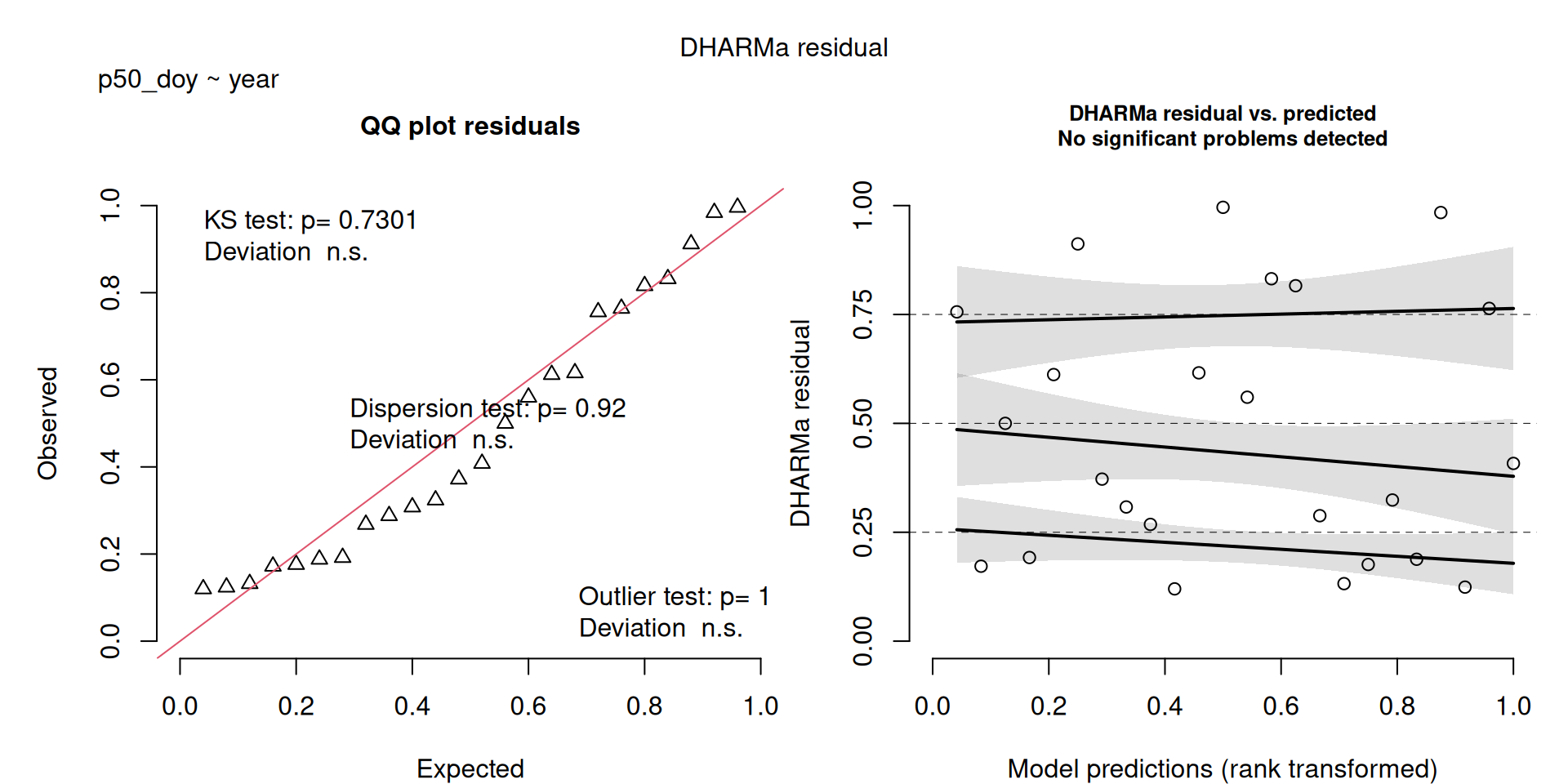
DHARMa plots
DHARMa is a package for simulating residuals to allow model checking for all types of models (details).
Generally these plots can be interpreted similarly to interpreting QQ Normal and Residual plots for linear models (although technically they’re using simulated residuals, not model residuals).
For context…
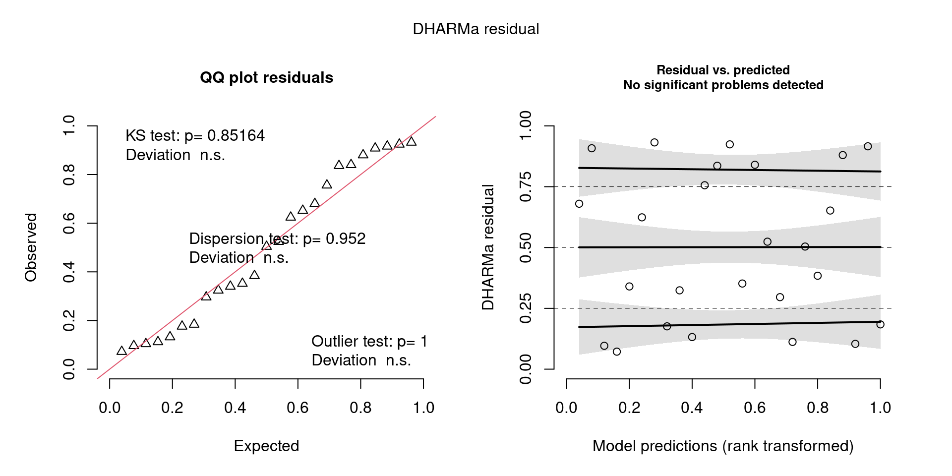
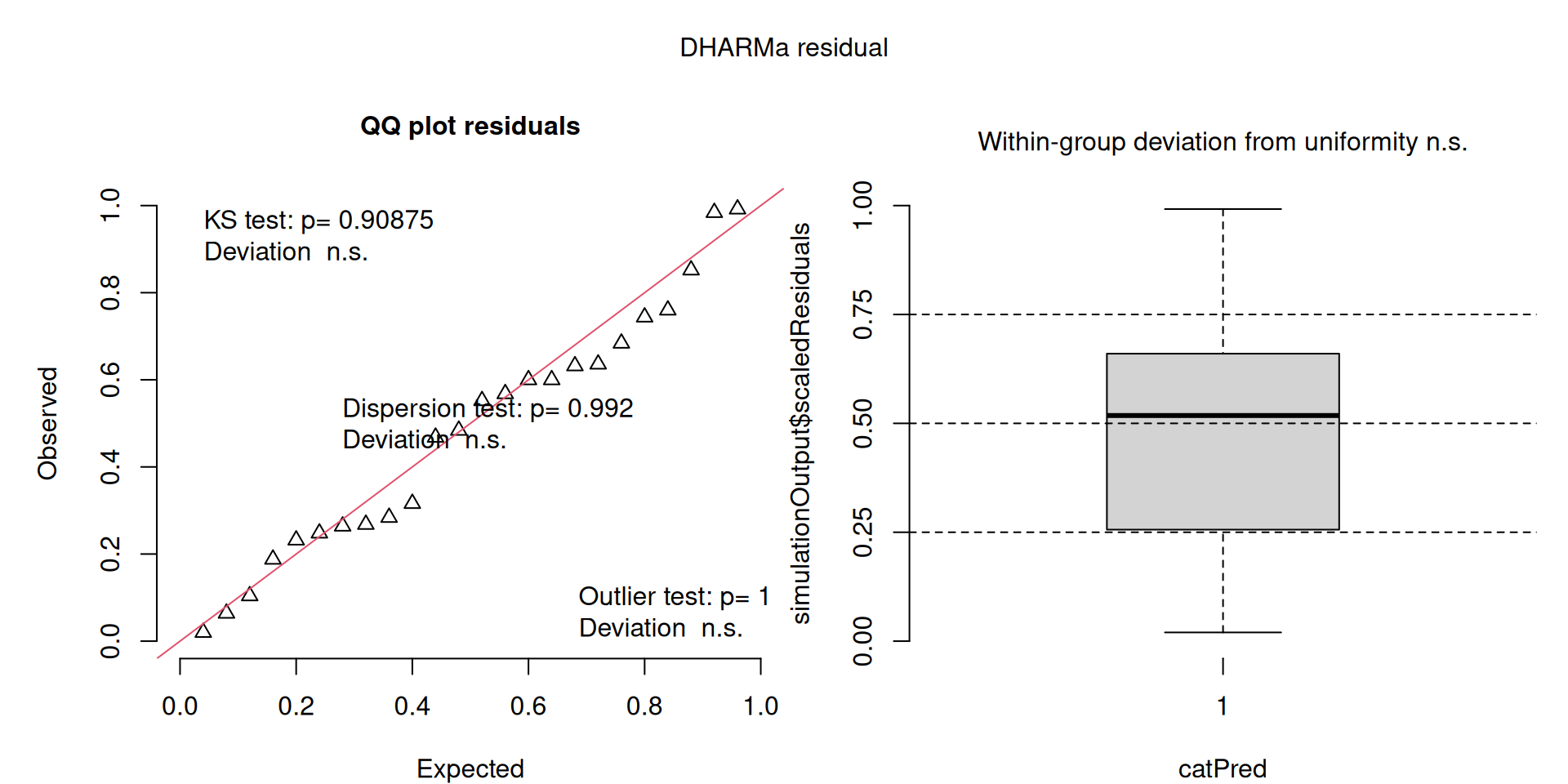
For example, we would interpret the following plot as showing decent model fit and assumptions.
The QQ plot on the left is nearly straight, there are no tests that flag problems in the distribution (KS test), Dispersion or Outliers. We also see no pattern in the residuals and no problems have been highlighted.
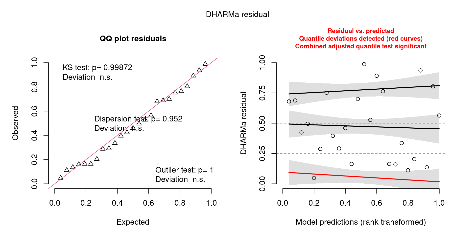
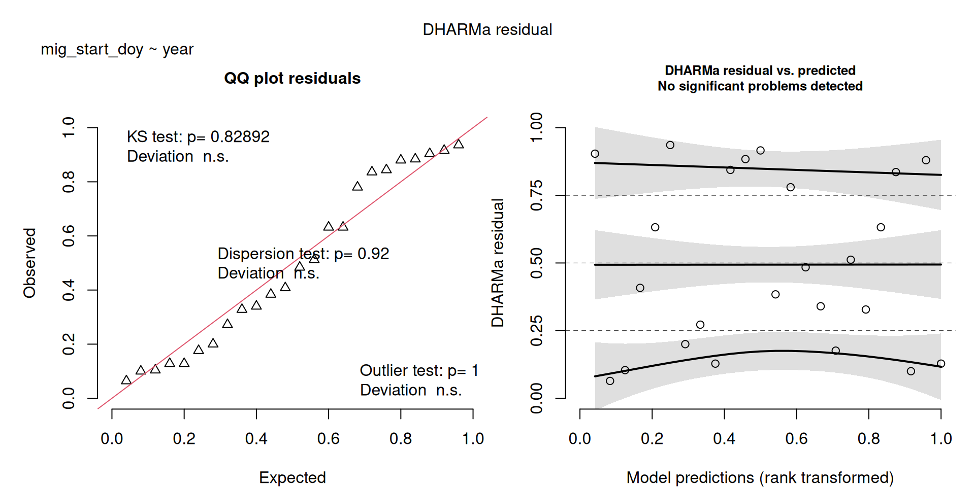
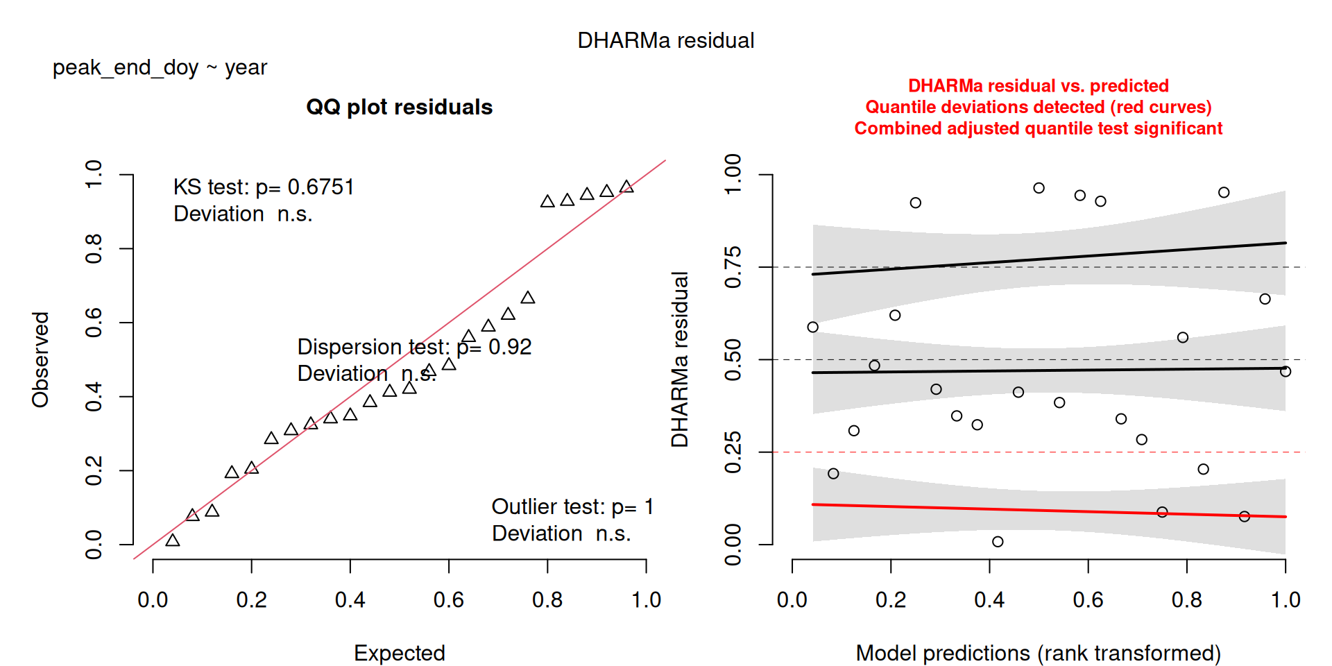
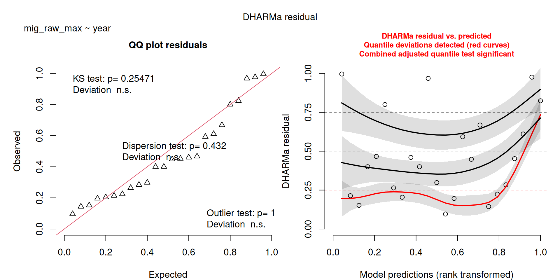
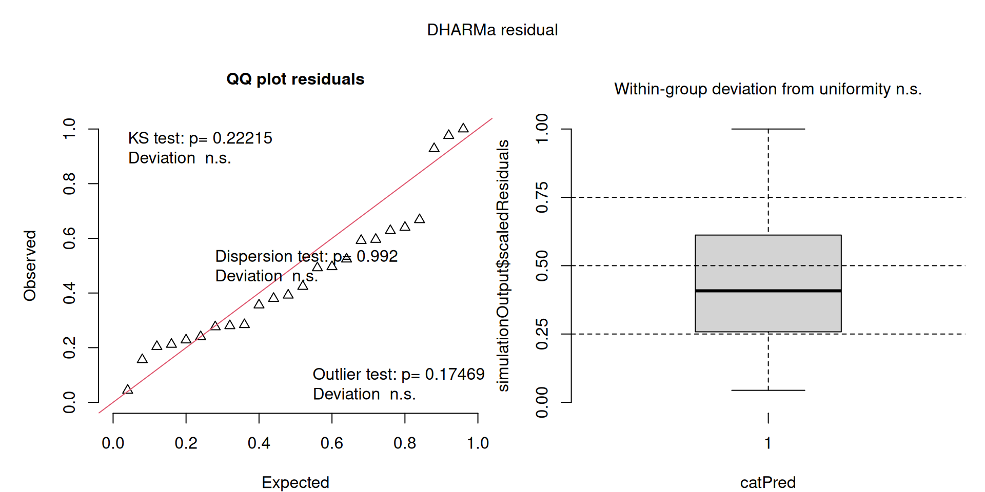
Similarly, I wouldn’t be unduly worried about the scary red line in this plot, as I don’t really find the residuals to show much pattern and there are no other problems highlighted.
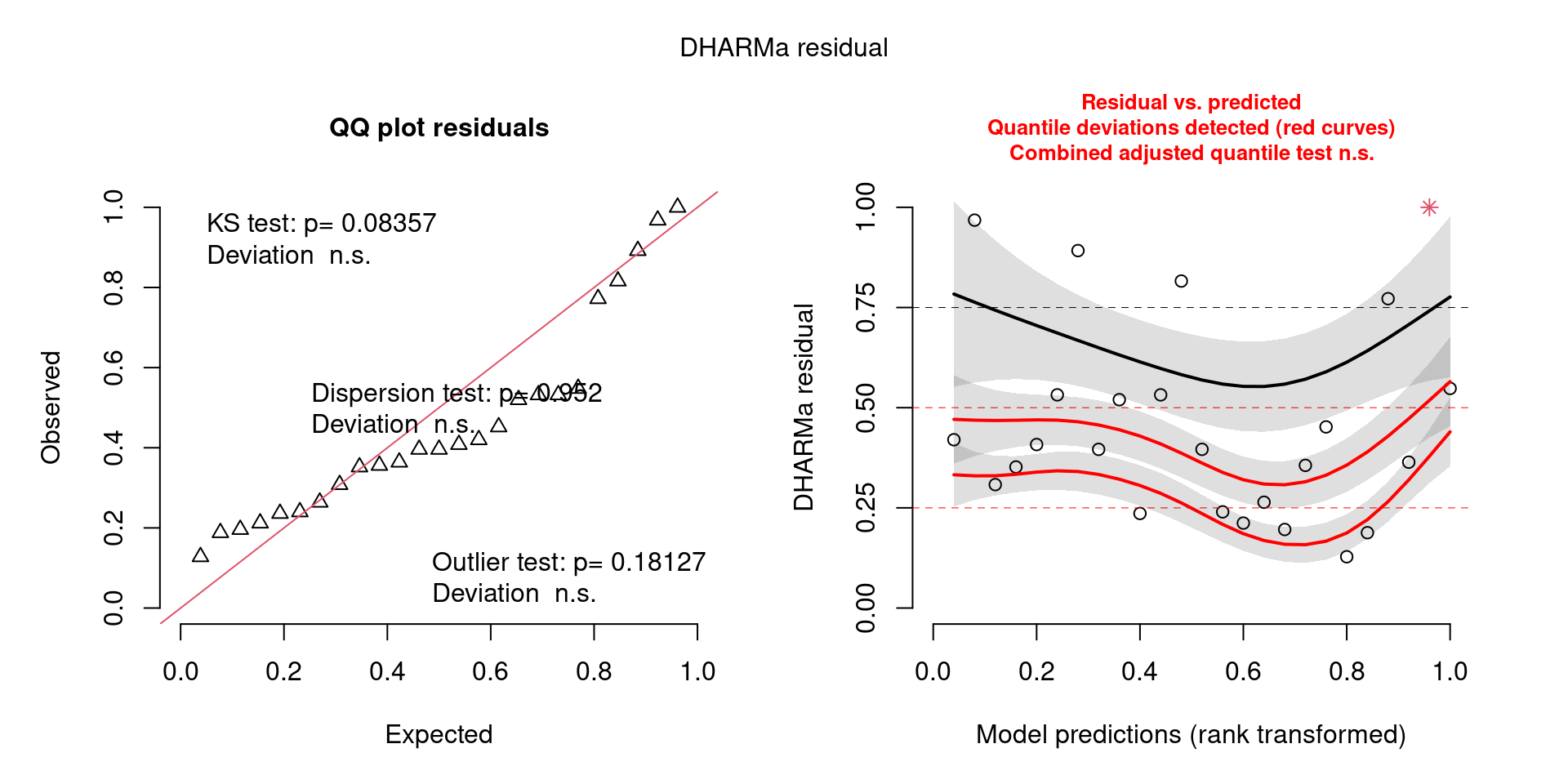
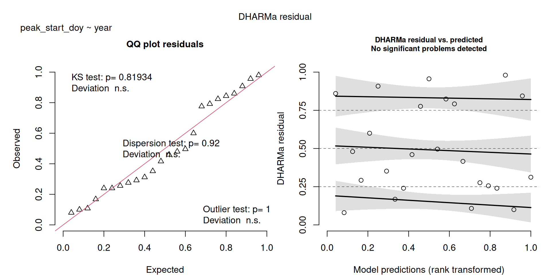
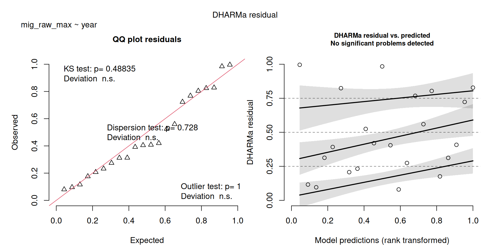
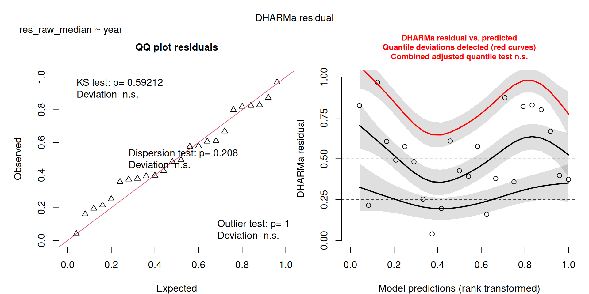
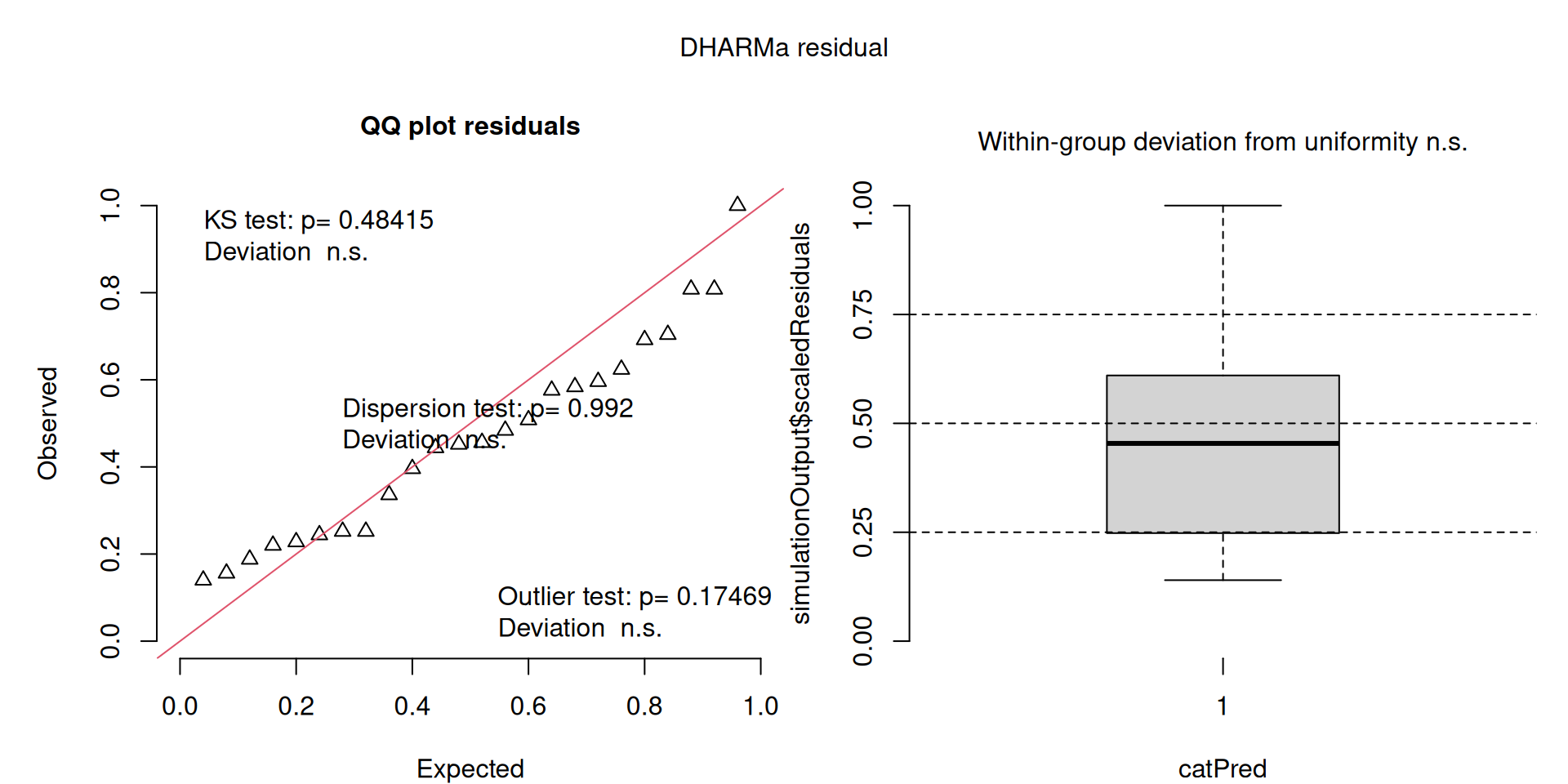
This one starts to look a bit problematic…
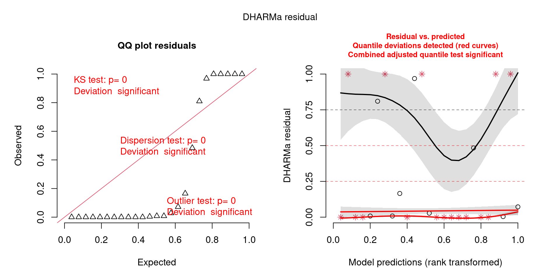
This one is awful!
Sensitivity
The DHARMa model checks will usually catch outlier problems, but out of an abundance of caution, we’ll do a quick review of any high Cook’s D values and will rerun the models without certain data points to ensure they’re still acceptable.
These sections first calculate and show the Cook’s D for all observations in each model. In these tables, values highlighted in red are more than 4/25 (a standard Cook’s D cutoff 4/sample size). These indicate potential influential data points for a particular model.
Then I run a comparison of the model before and the after removing that point.
In every case here the pattern was either strengthened or weakened by the removal, but the overall pattern did not change (no Estimate signs changed, and significance changed from sig to non-sig or vice versa).
- Strengthened patterns showed greater Estimates and smaller P values
- Weakened patterns showed smaller Estimates and greater P values
Tables with coefficients for both original and new model are shown, with colour intensity showing strength in the pattern.
Timing of kettle formation
When do kettles form? Has this timing changed over the years?
- Look for changes in the DOY of the 5%, 25%, 50%, 75%, 95%, of passage as well as the DOY with the highest predicted count.
mig_start_doy,peak_start_doy,p50_doy,peak_end_doy,mig_end_doy,max_doy
Descriptive stats
Day of Year
Code
v |>
  select(contains("start_doy"), contains("50_doy"), contains("end_doy"), "max_doy") |>
desc_stats()| measure | mean | sd | min | median | max | n |
|---|---|---|---|---|---|---|
| mig_start_doy | 259.50 | 3.02 | 253 | 259.5 | 265 | 24 |
| peak_start_doy | 266.88 | 2.31 | 262 | 267.0 | 272 | 24 |
| p50_doy | 271.62 | 2.32 | 268 | 271.0 | 277 | 24 |
| mig_end_doy | 283.79 | 3.08 | 277 | 284.0 | 289 | 24 |
| peak_end_doy | 276.42 | 2.34 | 272 | 276.0 | 281 | 24 |
| max_doy | 271.71 | 2.69 | 266 | 271.0 | 277 | 24 |
Date
Code
v |>
  select(contains("start_doy"), contains("50_doy"), contains("end_doy"), "max_doy") |>
desc_stats(units = "date")| measure | mean | sd | min | median | max | n |
|---|---|---|---|---|---|---|
| mig_start_doy | Sep 17 | 3.02 | Sep 10 | Sep 17 | Sep 22 | 24 |
| peak_start_doy | Sep 24 | 2.31 | Sep 19 | Sep 24 | Sep 29 | 24 |
| p50_doy | Sep 29 | 2.32 | Sep 25 | Sep 28 | Oct 04 | 24 |
| mig_end_doy | Oct 11 | 3.08 | Oct 04 | Oct 11 | Oct 16 | 24 |
| peak_end_doy | Oct 03 | 2.34 | Sep 29 | Oct 03 | Oct 08 | 24 |
| max_doy | Sep 29 | 2.69 | Sep 23 | Sep 28 | Oct 04 | 24 |
Here we look at linear regressions of year by kettle timing dates.
m1 <- lm(mig_start_doy ~ year, data = v)
m2 <- lm(peak_start_doy ~ year, data = v)
m3 <- lm(p50_doy ~ year, data = v)
m4 <- lm(peak_end_doy ~ year, data = v)
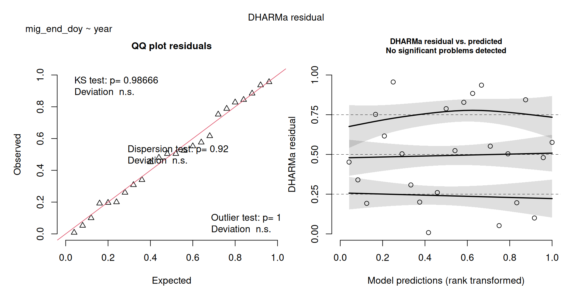
m5 <- lm(mig_end_doy ~ year, data = v)
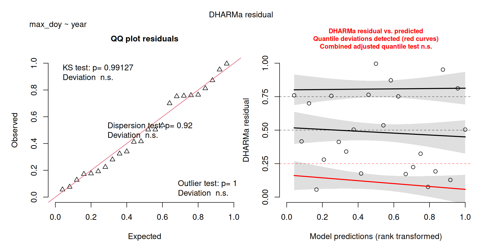
m6 <- lm(max_doy ~ year, data = v)
models <- list(m1, m2, m3, m4, m5, m6)Tabulated Model Results
All show a significant increase in doy except mig_end_doy. Data saved to Data/Datasets/table_timing.csv
Code
t1 <- get_table(models)
write_csv(t1, d)
fmt_table(t1)| term | estimate | std error | statistic | p value | n |
|---|---|---|---|---|---|
| mig_start_doy ~ year (R2 = 0.26; R2-adj = 0.23) | |||||
| (Intercept) | −155.793 | 149.151 | −1.045 | 0.308 | 24 |
| year | 0.206 | 0.074 | 2.784 | 0.011 | 24 |
| peak_start_doy ~ year (R2 = 0.33; R2-adj = 0.3) | |||||
| (Intercept) | −91.217 | 108.347 | −0.842 | 0.409 | 24 |
| year | 0.178 | 0.054 | 3.305 | 0.003 | 24 |
| p50_doy ~ year (R2 = 0.28; R2-adj = 0.25) | |||||
| (Intercept) | −58.259 | 112.980 | −0.516 | 0.611 | 24 |
| year | 0.164 | 0.056 | 2.920 | 0.008 | 24 |
| peak_end_doy ~ year (R2 = 0.25; R2-adj = 0.21) | |||||
| (Intercept) | −37.534 | 116.392 | −0.322 | 0.750 | 24 |
| year | 0.156 | 0.058 | 2.697 | 0.013 | 24 |
| mig_end_doy ~ year (R2 = 0.08; R2-adj = 0.04) | |||||
| (Intercept) | 44.280 | 169.169 | 0.262 | 0.796 | 24 |
| year | 0.119 | 0.084 | 1.416 | 0.171 | 24 |
| max_doy ~ year (R2 = 0.28; R2-adj = 0.25) | |||||
| (Intercept) | −110.936 | 131.392 | −0.844 | 0.408 | 24 |
| year | 0.190 | 0.065 | 2.912 | 0.008 | 24 |
Here we look at a linear regression of year by kettle timing dates. The idea is to explore whether the interaction is significant, which would indicate that the rate of change in migration phenology differs among the seasonal points (start, start of peak, peak, end of peak, end).
We look at the effect of year and type of measurement (migration start/end, peak start/end and time of 50% passage) on date (day of year).
Code
v1 <- select(v, ends_with("doy"), year) |>
  pivot_longer(-year, names_to = "measure", values_to = "doy")
First we look at the interaction term to see if the slopes of change among measurements are significantly different from one another.
The type III ANOVA shows no significant interaction.
Code
m0 <- lm(doy ~ measure * year, data = v1)
car::Anova(m0, type = "III")
Anova Table (Type III tests)
Response: doy
Sum Sq Df F value Pr(>F)
(Intercept) 3.90 1 0.6954 0.405829
measure 7.53 5 0.2681 0.929845
year 46.46 1 8.2739 0.004691 **
measure:year 5.93 5 0.2113 0.957236
Residuals 741.14 132
---
Signif. codes: 0 '***' 0.001 '**' 0.01 '*' 0.05 '.' 0.1 ' ' 1We’ll look at a post-hoc comparison of the slopes to interpret them individually.
This is nearly identical to running the models separately, above
As with the individual models, we can see that each measure shows a significant positive slope with the exception of the End of Migration (mig_end_day).
Code
e <- emmeans::emtrends(m0, ~ measure, var = "year") |>
  emmeans::test()
All show a significant increase in doy except mig_end_doy. Data saved to Data/Datasets/table_timing_combined.csv
Code
t2 <- e |>
  mutate(
    model = "doy ~ measure * year",
    n = nrow(v)) |>
  rename(
    estimate = year.trend,
    std_error = SE,

    statistic = t.ratio,
    p_value = p.value)

write_csv(t2, d)

fmt_table(t2) |>
  tab_header(title = "Post-hoc results") |>
  tab_footnote("Number of years in the data.", locations = cells_column_labels(n)) |>
tab_footnote("T statistic.", locations = cells_column_labels("statistic"))| Post-hoc results | ||||||
|---|---|---|---|---|---|---|
| measure | estimate | std error | df | statistic1 | p value | n2 |
| doy ~ measure * year | ||||||
| max_doy | 0.190 | 0.066 | 132 | 2.876 | 0.005 | 24 |
| mig_end_doy | 0.119 | 0.066 | 132 | 1.800 | 0.074 | 24 |
| mig_start_doy | 0.206 | 0.066 | 132 | 3.122 | 0.002 | 24 |
| p50_doy | 0.164 | 0.066 | 132 | 2.480 | 0.014 | 24 |
| peak_end_doy | 0.156 | 0.066 | 132 | 2.360 | 0.020 | 24 |
| peak_start_doy | 0.178 | 0.066 | 132 | 2.692 | 0.008 | 24 |
| 1 T statistic. | ||||||
| 2 Number of years in the data. | ||||||
Note: Lines without CI ribbons are not significant
Code
doy_figs <- v |>
  select(year, contains("doy")) |>
  pivot_longer(-year, names_to = "measure", values_to = "doy") |>
  left_join(mutate(t1, measure = str_trim(str_extract(model, "^[^~]*")), sig = p_value <= 0.05) |>
              filter(term == "year") |>
              select(measure, sig), by = "measure")

ggplot(doy_figs, aes(x = year, y = doy, group = measure, colour = measure, fill = sig)) +
  theme_bw() +
  geom_point() +
  geom_smooth(method = "lm", se = TRUE) +
  scale_y_continuous(breaks = y_breaks) +
  scale_colour_viridis_d() +
  scale_fill_manual(values = c("TRUE" = "grey60", "FALSE" = "#FFFFFF00"), guide = "none") +
  labs(caption = "Lines without CI Error ribbons represent non-significant models")
`geom_smooth()` using formula = 'y ~ x'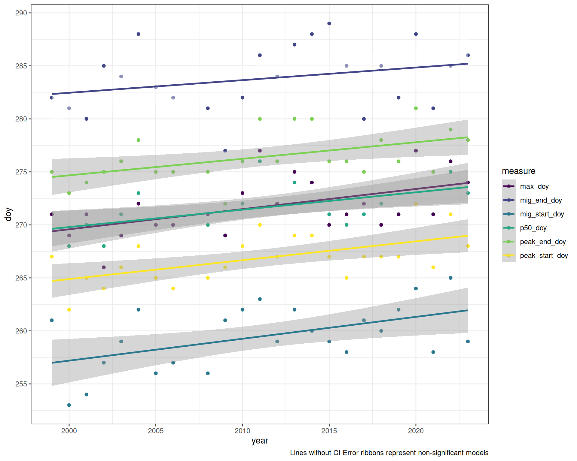
The DHARMa model checks don’t highlight any particular outlier problems, but out of an abundance of caution, we’ll do a quick review of any high Cook’s D values.
Values highlighted in red are more than 4/25, a standard Cook’s D cutoff (4/sample size). These indicate potential influential data points for a particular model.
Code
get_cooks(models) |>
gt_cooks(width = "80%")| Cook's Distances | ||||||
|---|---|---|---|---|---|---|
| year | mig_start_doy | peak_start_doy | p50_doy | peak_end_doy | mig_end_doy | max_doy |
| 1999 | 0.25 | 0.16 | 0.05 | 0.01 | 0.00 | 0.05 |
| 2000 | 0.23 | 0.21 | 0.07 | 0.06 | 0.02 | 0.01 |
| 2001 | 0.13 | 0.00 | 0.00 | 0.01 | 0.06 | 0.02 |
| 2002 | 0.00 | 0.03 | 0.07 | 0.00 | 0.04 | 0.19 |
| 2003 | 0.01 | 0.01 | 0.01 | 0.01 | 0.01 | 0.01 |
| 2004 | 0.11 | 0.07 | 0.08 | 0.08 | 0.14 | 0.02 |
| 2005 | 0.03 | 0.01 | 0.00 | 0.00 | 0.00 | 0.00 |
| 2006 | 0.01 | 0.04 | 0.01 | 0.00 | 0.01 | 0.00 |
| 2008 | 0.03 | 0.01 | 0.01 | 0.01 | 0.02 | 0.00 |
| 2009 | 0.01 | 0.00 | 0.03 | 0.10 | 0.12 | 0.02 |
| 2010 | 0.02 | 0.01 | 0.00 | 0.00 | 0.01 | 0.01 |
| 2011 | 0.04 | 0.06 | 0.11 | 0.07 | 0.01 | 0.12 |
| 2012 | 0.00 | 0.00 | 0.00 | 0.00 | 0.00 | 0.00 |
| 2013 | 0.02 | 0.02 | 0.03 | 0.06 | 0.02 | 0.04 |
| 2014 | 0.00 | 0.02 | 0.02 | 0.06 | 0.04 | 0.01 |
| 2015 | 0.01 | 0.00 | 0.01 | 0.01 | 0.07 | 0.03 |
| 2016 | 0.03 | 0.07 | 0.05 | 0.01 | 0.00 | 0.02 |
| 2017 | 0.00 | 0.01 | 0.02 | 0.05 | 0.09 | 0.00 |
| 2018 | 0.01 | 0.01 | 0.01 | 0.00 | 0.00 | 0.08 |
| 2019 | 0.01 | 0.02 | 0.05 | 0.03 | 0.04 | 0.05 |
| 2020 | 0.06 | 0.22 | 0.24 | 0.15 | 0.07 | 0.15 |
| 2021 | 0.13 | 0.14 | 0.09 | 0.15 | 0.13 | 0.09 |
| 2022 | 0.13 | 0.11 | 0.06 | 0.02 | 0.00 | 0.08 |
| 2023 | 0.13 | 0.03 | 0.01 | 0.00 | 0.01 | 0.00 |
Check influential points
Now let’s see what happens if we were to omit these years from the respective analyses.
Tables with coefficients for both original and new model are shown, with colour intensity showing strength in the pattern.
For the start of migration, if we omit 1999, the pattern is stronger, but the same, if we omit 2000, the pattern is weaker but still the same.
compare(m1, 1999)| model | parameter | Estimate | Std. Error | t value | Pr(>|t|) |
|---|---|---|---|---|---|
| Original - mig_start_doy | (Intercept) | -155.793 | 149.151 | -1.045 | 0.308 |
| Drop 1999 - mig_start_doy | (Intercept) | -246.743 | 152.473 | -1.618 | 0.121 |
| Original - mig_start_doy | year | 0.206 | 0.074 | 2.784 | 0.011 |
| Drop 1999 - mig_start_doy | year | 0.252 | 0.076 | 3.320 | 0.003 |
compare(m1, 2000)| model | parameter | Estimate | Std. Error | t value | Pr(>|t|) |
|---|---|---|---|---|---|
| Original - mig_start_doy | (Intercept) | -155.793 | 149.151 | -1.045 | 0.308 |
| Drop 2000 - mig_start_doy | (Intercept) | -70.361 | 150.113 | -0.469 | 0.644 |
| Original - mig_start_doy | year | 0.206 | 0.074 | 2.784 | 0.011 |
| Drop 2000 - mig_start_doy | year | 0.164 | 0.075 | 2.199 | 0.039 |
For the start of peak migration
compare(m2, 2000)| model | parameter | Estimate | Std. Error | t value | Pr(>|t|) |
|---|---|---|---|---|---|
| Original - peak_start_doy | (Intercept) | -91.217 | 108.347 | -0.842 | 0.409 |
| Drop 2000 - peak_start_doy | (Intercept) | -32.416 | 109.888 | -0.295 | 0.771 |
| Original - peak_start_doy | year | 0.178 | 0.054 | 3.305 | 0.003 |
| Drop 2000 - peak_start_doy | year | 0.149 | 0.055 | 2.726 | 0.013 |
compare(m2, 2020)| model | parameter | Estimate | Std. Error | t value | Pr(>|t|) |
|---|---|---|---|---|---|
| Original - peak_start_doy | (Intercept) | -91.217 | 108.347 | -0.842 | 0.409 |
| Drop 2020 - peak_start_doy | (Intercept) | -36.595 | 104.279 | -0.351 | 0.729 |
| Original - peak_start_doy | year | 0.178 | 0.054 | 3.305 | 0.003 |
| Drop 2020 - peak_start_doy | year | 0.151 | 0.052 | 2.908 | 0.008 |
The date of 50% passage
compare(m3, 2020)| model | parameter | Estimate | Std. Error | t value | Pr(>|t|) |
|---|---|---|---|---|---|
| Original - p50_doy | (Intercept) | -58.259 | 112.980 | -0.516 | 0.611 |
| Drop 2020 - p50_doy | (Intercept) | 2.113 | 107.339 | 0.020 | 0.984 |
| Original - p50_doy | year | 0.164 | 0.056 | 2.920 | 0.008 |
| Drop 2020 - p50_doy | year | 0.134 | 0.053 | 2.509 | 0.020 |
And the date of maximum counts
compare(m6, 2002)| model | parameter | Estimate | Std. Error | t value | Pr(>|t|) |
|---|---|---|---|---|---|
| Original - max_doy | (Intercept) | -110.936 | 131.392 | -0.844 | 0.408 |
| Drop 2002 - max_doy | (Intercept) | -46.968 | 128.776 | -0.365 | 0.719 |
| Original - max_doy | year | 0.190 | 0.065 | 2.912 | 0.008 |
| Drop 2002 - max_doy | year | 0.159 | 0.064 | 2.477 | 0.022 |
In addition to the sensitivity check using cook’s distances, here we will conduct a more targeted exploration of some specific years.
Gaps around the peak
First, we consider removing 2011, 2013 as they have sampling gaps around the peak of migration
y <- c(2011, 2013)
m1a <- update(m1, data = filter(v, !year %in% y))
m2a <- update(m2, data = filter(v, !year %in% y))
m3a <- update(m3, data = filter(v, !year %in% y))
m4a <- update(m4, data = filter(v, !year %in% y))
m5a <- update(m5, data = filter(v, !year %in% y))
m6a <- update(m6, data = filter(v, !year %in% y))

models_a <- list(m1a, m2a, m3a, m4a, m5a, m6a)
Comparing the summary tables shows only superficial differences. If anything, it looks like removing these ‘gappy’ years only strengthens the existing patterns. Those which are significant are slightly more so, and the slopes are slightly greater.
Data saved to Data/Datasets/table_supplemental.csv
Original
Code
fmt_summary(models, intercept = FALSE)| model | Parameter | Estimate | Std. Error | T | P |
|---|---|---|---|---|---|
| mig_start_doy ~ year | year | 0.206 | 0.074 | 2.784 | 0.011 |
| peak_start_doy ~ year | year | 0.178 | 0.054 | 3.305 | 0.003 |
| p50_doy ~ year | year | 0.164 | 0.056 | 2.920 | 0.008 |
| peak_end_doy ~ year | year | 0.156 | 0.058 | 2.697 | 0.013 |
| mig_end_doy ~ year | year | 0.119 | 0.084 | 1.416 | 0.171 |
| max_doy ~ year | year | 0.190 | 0.065 | 2.912 | 0.008 |
Code
to <- get_table(models) |>
  select(model, term, estimate, std_error, statistic, p_value) |>
  mutate(type = "original")
write_csv(to, d)
Years removed
Code
fmt_summary(models_a, intercept = FALSE)| model | Parameter | Estimate | Std. Error | T | P |
|---|---|---|---|---|---|
| mig_start_doy ~ year | year | 0.204 | 0.073 | 2.784 | 0.011 |
| peak_start_doy ~ year | year | 0.176 | 0.051 | 3.416 | 0.003 |
| p50_doy ~ year | year | 0.161 | 0.050 | 3.237 | 0.004 |
| peak_end_doy ~ year | year | 0.151 | 0.052 | 2.928 | 0.008 |
| mig_end_doy ~ year | year | 0.115 | 0.085 | 1.352 | 0.192 |
| max_doy ~ year | year | 0.186 | 0.056 | 3.324 | 0.003 |
Code
ta <- get_table(models_a) |>
  select(model, term, estimate, std_error, statistic, p_value) |>
  mutate(type = "gaps_removed")
write_csv(ta, d, append = TRUE)
Missing the end of migration
Second, we consider removing 2001, 2006, 2023 as they were three years where it looks like sampling ended earlier than the end of migration.
y <- c(2001, 2006, 2023)
m1b <- update(m1, data = filter(v, !year %in% y))
m2b <- update(m2, data = filter(v, !year %in% y))
m3b <- update(m3, data = filter(v, !year %in% y))
m4b <- update(m4, data = filter(v, !year %in% y))
m5b <- update(m5, data = filter(v, !year %in% y))
m6b <- update(m6, data = filter(v, !year %in% y))

models_b <- list(m1b, m2b, m3b, m4b, m5b, m6b)
Removing these years from the analyses, reduced the strength of the patterns, but not by much. Further, there were few changes to the magnitude of the slopes.
Data saved to Data/Datasets/table_supplemental.csv
Original
Code
fmt_summary(models, intercept = FALSE)| model | Parameter | Estimate | Std. Error | T | P |
|---|---|---|---|---|---|
| mig_start_doy ~ year | year | 0.206 | 0.074 | 2.784 | 0.011 |
| peak_start_doy ~ year | year | 0.178 | 0.054 | 3.305 | 0.003 |
| p50_doy ~ year | year | 0.164 | 0.056 | 2.920 | 0.008 |
| peak_end_doy ~ year | year | 0.156 | 0.058 | 2.697 | 0.013 |
| mig_end_doy ~ year | year | 0.119 | 0.084 | 1.416 | 0.171 |
| max_doy ~ year | year | 0.190 | 0.065 | 2.912 | 0.008 |
Years removed
Code
fmt_summary(models_b, intercept = FALSE)| model | Parameter | Estimate | Std. Error | T | P |
|---|---|---|---|---|---|
| mig_start_doy ~ year | year | 0.198 | 0.082 | 2.410 | 0.026 |
| peak_start_doy ~ year | year | 0.178 | 0.063 | 2.825 | 0.011 |
| p50_doy ~ year | year | 0.167 | 0.068 | 2.467 | 0.023 |
| peak_end_doy ~ year | year | 0.147 | 0.070 | 2.119 | 0.048 |
| mig_end_doy ~ year | year | 0.077 | 0.099 | 0.781 | 0.445 |
| max_doy ~ year | year | 0.198 | 0.078 | 2.530 | 0.020 |
Code
tb <- get_table(models_b) |>
  select(model, term, estimate, std_error, statistic, p_value) |>
  mutate(type = "end_removed")
write_csv(tb, d, append = TRUE)
Remove all problematic years
Out of curiosity, let’s try removing all 5 years. This reduces our data from 25 to 19 samples, so is a substantial change and we may see non-significant results merely because we have removed too many samples.
y <- c(2011, 2013, 2001, 2006, 2023)
m1c <- update(m1, data = filter(v, !year %in% y))
m2c <- update(m2, data = filter(v, !year %in% y))
m3c <- update(m3, data = filter(v, !year %in% y))
m4c <- update(m4, data = filter(v, !year %in% y))
m5c <- update(m5, data = filter(v, !year %in% y))
m6c <- update(m6, data = filter(v, !year %in% y))

models_c <- list(m1c, m2c, m3c, m4c, m5c, m6c)
Removing these years from the analyses, reduced the strength of the patterns, but not by much. Further, there are few changes to the magnitude of the slopes.
Data saved to Data/Datasets/table_supplemental.csv
Original
Code
fmt_summary(models, intercept = FALSE)| model | Parameter | Estimate | Std. Error | T | P |
|---|---|---|---|---|---|
| mig_start_doy ~ year | year | 0.206 | 0.074 | 2.784 | 0.011 |
| peak_start_doy ~ year | year | 0.178 | 0.054 | 3.305 | 0.003 |
| p50_doy ~ year | year | 0.164 | 0.056 | 2.920 | 0.008 |
| peak_end_doy ~ year | year | 0.156 | 0.058 | 2.697 | 0.013 |
| mig_end_doy ~ year | year | 0.119 | 0.084 | 1.416 | 0.171 |
| max_doy ~ year | year | 0.190 | 0.065 | 2.912 | 0.008 |
Years removed
Code
fmt_summary(models_c, intercept = FALSE)| model | Parameter | Estimate | Std. Error | T | P |
|---|---|---|---|---|---|
| mig_start_doy ~ year | year | 0.196 | 0.082 | 2.387 | 0.029 |
| peak_start_doy ~ year | year | 0.176 | 0.061 | 2.893 | 0.010 |
| p50_doy ~ year | year | 0.165 | 0.061 | 2.715 | 0.015 |
| peak_end_doy ~ year | year | 0.143 | 0.063 | 2.270 | 0.036 |
| mig_end_doy ~ year | year | 0.073 | 0.101 | 0.722 | 0.480 |
| max_doy ~ year | year | 0.195 | 0.067 | 2.901 | 0.010 |
Code
tc <- get_table(models_c) |>
  select(model, term, estimate, std_error, statistic, p_value) |>
  mutate(type = "all_removed")
write_csv(tc, d, append = TRUE)
Conclusions
I do not believe that these potentially problematic sampling years are driving the patterns we see in this data.
At worst, by removing these years we increase the error around a slope. But the magnitudes of the slopes do not change very much and even the significance is only ever reduced only a little.
Code
models <- append(list(m0), models)
map(models, summary)
[[1]]
Call:
lm(formula = doy ~ measure * year, data = v1)
Residuals:
Min 1Q Median 3Q Max
-6.5336 -1.5933 -0.3033 1.6795 5.3234
Coefficients:
Estimate Std. Error t value Pr(>|t|)
(Intercept) -110.93571 133.02821 -0.834 0.40583
measuremig_end_doy 155.21571 188.13030 0.825 0.41084
measuremig_start_doy -44.85714 188.13030 -0.238 0.81191
measurep50_doy 52.67714 188.13030 0.280 0.77991
measurepeak_end_doy 73.40143 188.13030 0.390 0.69705
measurepeak_start_doy 19.71857 188.13030 0.105 0.91668
year 0.19026 0.06614 2.876 0.00469 **
measuremig_end_doy:year -0.07117 0.09354 -0.761 0.44812
measuremig_start_doy:year 0.01623 0.09354 0.174 0.86249
measurep50_doy:year -0.02623 0.09354 -0.280 0.77957
measurepeak_end_doy:year -0.03416 0.09354 -0.365 0.71559
measurepeak_start_doy:year -0.01221 0.09354 -0.131 0.89637
---
Signif. codes: 0 '***' 0.001 '**' 0.01 '*' 0.05 '.' 0.1 ' ' 1
Residual standard error: 2.37 on 132 degrees of freedom
Multiple R-squared: 0.9189, Adjusted R-squared: 0.9122
F-statistic: 136 on 11 and 132 DF, p-value: < 2.2e-16
[[2]]
Call:
lm(formula = mig_start_doy ~ year, data = v)
Residuals:
Min 1Q Median 3Q Max
-4.1942 -2.2945 -0.3461 2.2601 4.0123
Coefficients:
Estimate Std. Error t value Pr(>|t|)
(Intercept) -155.79286 149.15112 -1.045 0.3076
year 0.20649 0.07416 2.784 0.0108 *
---
Signif. codes: 0 '***' 0.001 '**' 0.01 '*' 0.05 '.' 0.1 ' ' 1
Residual standard error: 2.657 on 22 degrees of freedom
Multiple R-squared: 0.2606, Adjusted R-squared: 0.227
F-statistic: 7.753 on 1 and 22 DF, p-value: 0.01081
[[3]]
Call:
lm(formula = peak_start_doy ~ year, data = v)
Residuals:
Min 1Q Median 3Q Max
-2.8868 -1.2496 -0.5234 1.6650 3.5522
Coefficients:
Estimate Std. Error t value Pr(>|t|)
(Intercept) -91.21714 108.34732 -0.842 0.40891
year 0.17805 0.05387 3.305 0.00322 **
---
Signif. codes: 0 '***' 0.001 '**' 0.01 '*' 0.05 '.' 0.1 ' ' 1
Residual standard error: 1.93 on 22 degrees of freedom
Multiple R-squared: 0.3318, Adjusted R-squared: 0.3014
F-statistic: 10.92 on 1 and 22 DF, p-value: 0.003223
[[4]]
Call:
lm(formula = p50_doy ~ year, data = v)
Residuals:
Min 1Q Median 3Q Max
-2.4178 -1.6347 -0.5897 1.4275 4.4023
Coefficients:
Estimate Std. Error t value Pr(>|t|)
(Intercept) -58.25857 112.98029 -0.516 0.61124
year 0.16403 0.05618 2.920 0.00794 **
---
Signif. codes: 0 '***' 0.001 '**' 0.01 '*' 0.05 '.' 0.1 ' ' 1
Residual standard error: 2.012 on 22 degrees of freedom
Multiple R-squared: 0.2793, Adjusted R-squared: 0.2465
F-statistic: 8.526 on 1 and 22 DF, p-value: 0.007935
[[5]]
Call:
lm(formula = peak_end_doy ~ year, data = v)
Residuals:
Min 1Q Median 3Q Max
-4.0784 -1.0541 -0.3590 0.8667 3.6094
Coefficients:
Estimate Std. Error t value Pr(>|t|)
(Intercept) -37.53429 116.39244 -0.322 0.7501
year 0.15610 0.05787 2.697 0.0132 *
---
Signif. codes: 0 '***' 0.001 '**' 0.01 '*' 0.05 '.' 0.1 ' ' 1
Residual standard error: 2.073 on 22 degrees of freedom
Multiple R-squared: 0.2485, Adjusted R-squared: 0.2144
F-statistic: 7.276 on 1 and 22 DF, p-value: 0.01316
[[6]]
Call:
lm(formula = mig_end_doy ~ year, data = v)
Residuals:
Min 1Q Median 3Q Max
-6.5336 -1.8432 0.0259 2.2461 5.0618
Coefficients:
Estimate Std. Error t value Pr(>|t|)
(Intercept) 44.28000 169.16915 0.262 0.796
year 0.11909 0.08411 1.416 0.171
Residual standard error: 3.013 on 22 degrees of freedom
Multiple R-squared: 0.08351, Adjusted R-squared: 0.04185
F-statistic: 2.005 on 1 and 22 DF, p-value: 0.1708
[[7]]
Call:
lm(formula = max_doy ~ year, data = v)
Residuals:
Min 1Q Median 3Q Max
-3.9643 -1.7706 -0.3205 1.6187 5.3234
Coefficients:
Estimate Std. Error t value Pr(>|t|)
(Intercept) -110.93571 131.39209 -0.844 0.40758
year 0.19026 0.06533 2.912 0.00808 **
---
Signif. codes: 0 '***' 0.001 '**' 0.01 '*' 0.05 '.' 0.1 ' ' 1
Residual standard error: 2.34 on 22 degrees of freedom
Multiple R-squared: 0.2782, Adjusted R-squared: 0.2454
F-statistic: 8.481 on 1 and 22 DF, p-value: 0.008075Code
model_check_figs(models)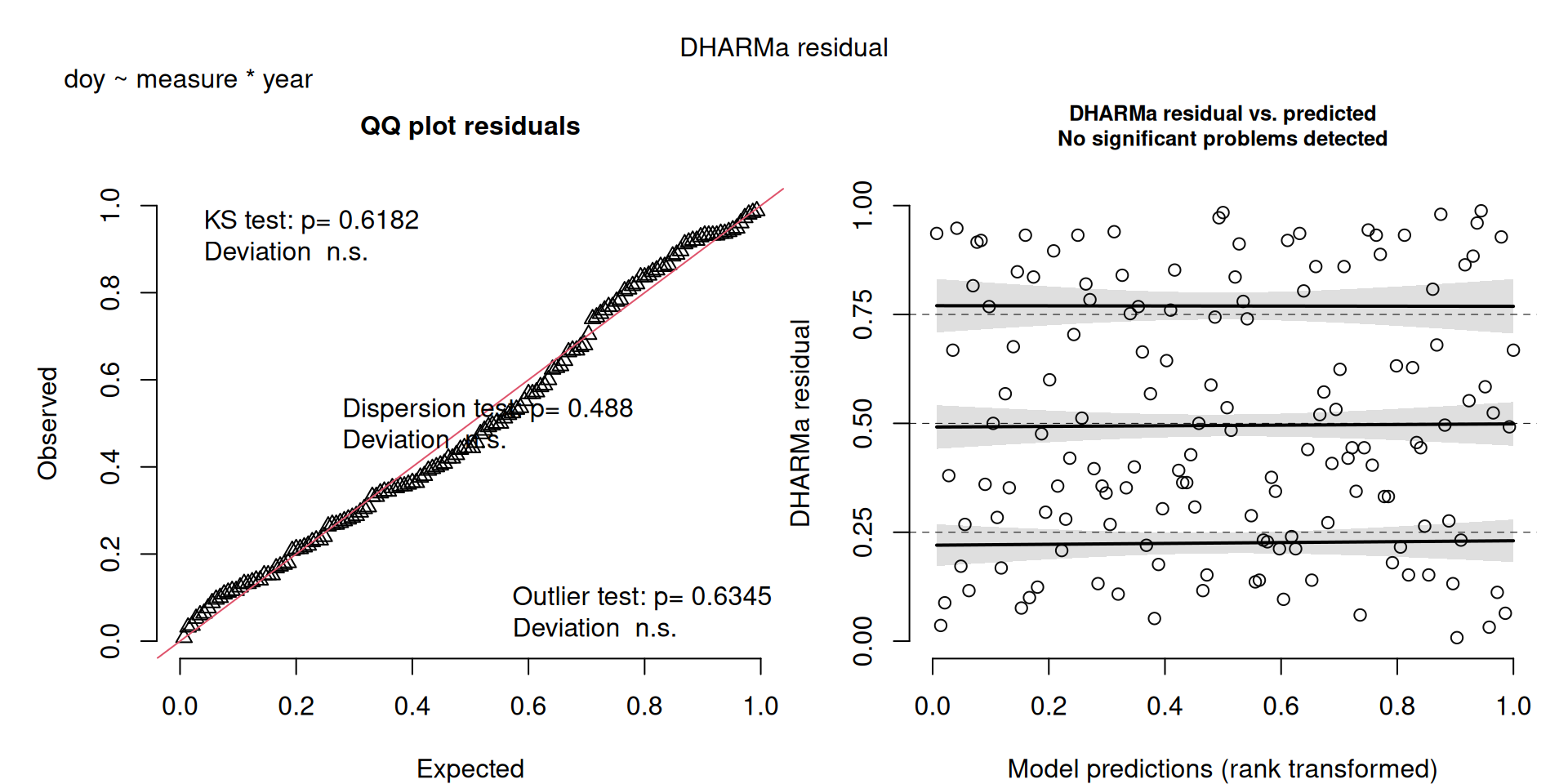
Duration of migration
How long is migration? Has it changed in length?
- Look for changes in the number of days over which migration and peak migration occur
mig_dur_days,peak_dur_days
Descriptive stats
Code
v |>
  select(contains("dur")) |>
desc_stats()| measure | mean | sd | min | median | max | n |
|---|---|---|---|---|---|---|
| mig_dur_days | 24.29 | 3.43 | 16 | 25 | 30 | 24 |
| peak_dur_days | 9.54 | 1.32 | 6 | 10 | 11 | 24 |
m1 <- lm(mig_dur_days ~ year, data = v)
m2 <- lm(peak_dur_days ~ year, data = v)

models <- list(m1, m2)
Tabulated Results
No significant results
Code
t <- get_table(models)
write_csv(t, "Data/Datasets/table_duration.csv")
fmt_table(t)| term | estimate | std error | statistic | p value | n |
|---|---|---|---|---|---|
| mig_dur_days ~ year (R2 = 0.04; R2-adj = -0.01) | |||||
| (Intercept) | 200.073 | 193.428 | 1.034 | 0.312 | 24 |
| year | −0.087 | 0.096 | −0.909 | 0.373 | 24 |
| peak_dur_days ~ year (R2 = 0.02; R2-adj = -0.03) | |||||
| (Intercept) | 53.683 | 75.074 | 0.715 | 0.482 | 24 |
| year | −0.022 | 0.037 | −0.588 | 0.563 | 24 |
Note: Lines without Std Error ribbons are not significant
Code
dur_figs <- v |>
  select(year, contains("dur")) |>
  pivot_longer(-year, names_to = "measure", values_to = "dur")

ggplot(dur_figs, aes(x = year, y = dur, group = measure, colour = measure)) +
  theme_bw() +
  geom_point() +
  stat_smooth(method = "lm", se = FALSE) +
  #scale_y_continuous(breaks = y_breaks) +
  scale_colour_viridis_d()+
  labs(caption = "Lines without Std Error ribbons represent non-significant models")
`geom_smooth()` using formula = 'y ~ x'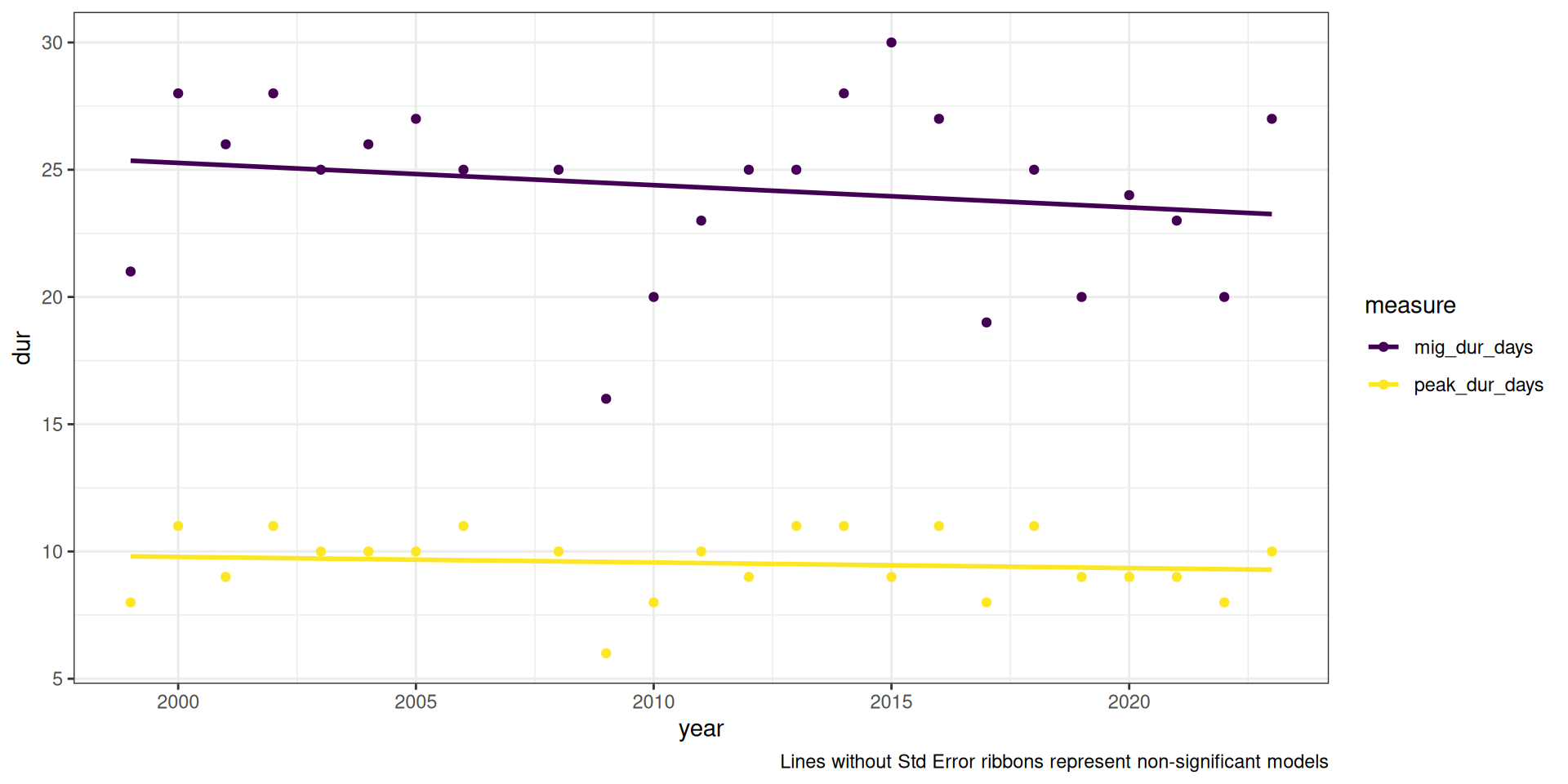
Some pattern to the upper quandrant residuals, but I think the more reflects what we’re seeing, that year is a poor predictor of migration duration.
Code
model_check_figs(models)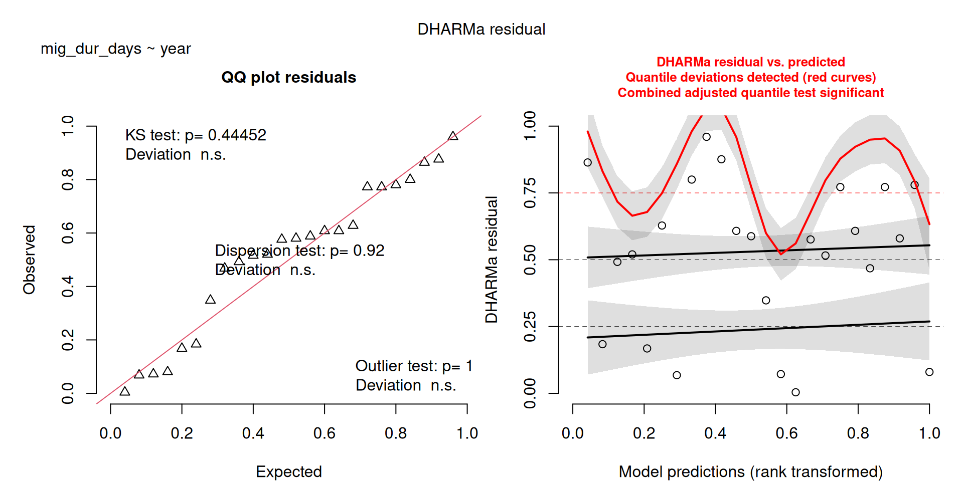
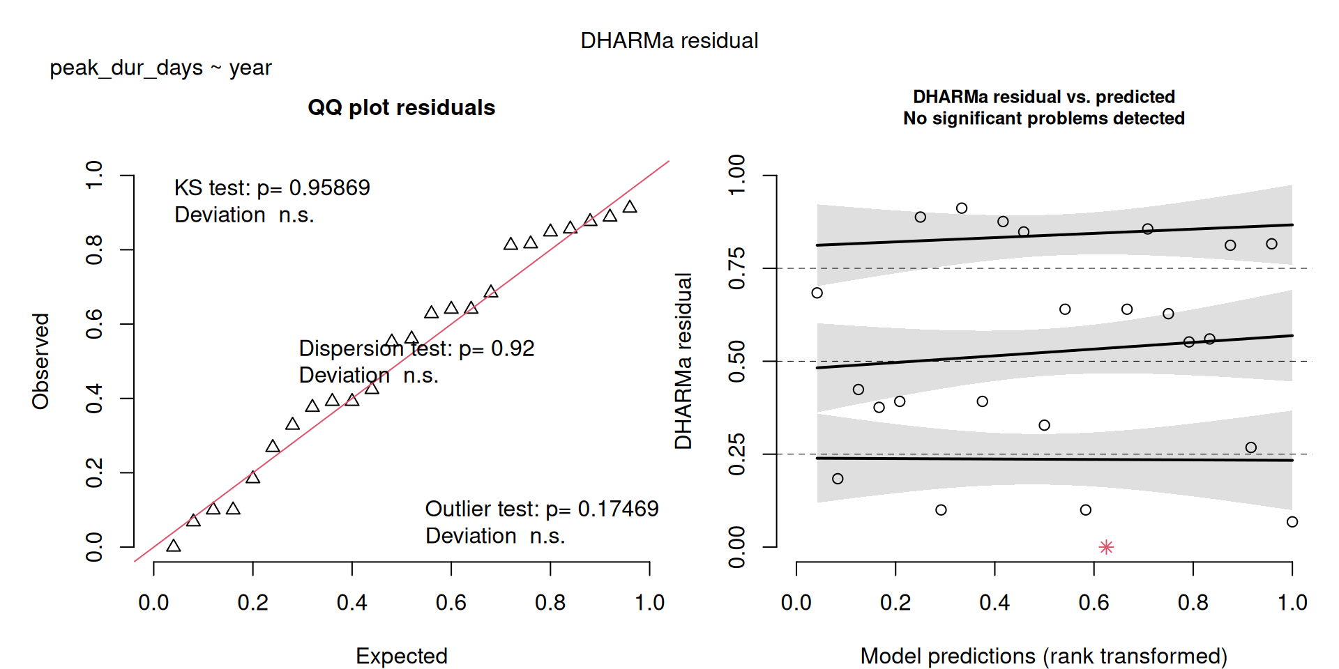
The DHARMa model checks don’t highlight any particular outlier problems, but out of an abundance of caution, we’ll do a quick review of any high Cook’s D values.
Values highlighted in red are more than 4/25, a standard Cook’s D cutoff (4/sample size). These indicate potential influential data points for a particular model.
Code
get_cooks(models) |>
gt_cooks()| Cook's Distances | ||
|---|---|---|
| year | mig_dur_days | peak_dur_days |
| 1999 | 0.18 | 0.20 |
| 2000 | 0.06 | 0.08 |
| 2001 | 0.00 | 0.03 |
| 2002 | 0.05 | 0.06 |
| 2003 | 0.00 | 0.00 |
| 2004 | 0.00 | 0.00 |
| 2005 | 0.02 | 0.00 |
| 2006 | 0.00 | 0.04 |
| 2008 | 0.00 | 0.00 |
| 2009 | 0.15 | 0.18 |
| 2010 | 0.04 | 0.03 |
| 2011 | 0.00 | 0.00 |
| 2012 | 0.00 | 0.00 |
| 2013 | 0.00 | 0.03 |
| 2014 | 0.03 | 0.03 |
| 2015 | 0.09 | 0.00 |
| 2016 | 0.03 | 0.05 |
| 2017 | 0.08 | 0.04 |
| 2018 | 0.01 | 0.07 |
| 2019 | 0.06 | 0.00 |
| 2020 | 0.00 | 0.00 |
| 2021 | 0.00 | 0.00 |
| 2022 | 0.08 | 0.08 |
| 2023 | 0.12 | 0.03 |
Check influential points
Now let’s see what happens if we were to omit these years from the respective analyses.
Tables with coefficients for both original and new model are shown, with colour intensity showing strength in the pattern.
For the number of days in peak migration, if we omit 1999, the pattern is stronger, but the same (i.e. not significant), we see the same for the number of days in peak migration for 1999 and 2009.
compare(m1, 1999)| model | parameter | Estimate | Std. Error | t value | Pr(>|t|) |
|---|---|---|---|---|---|
| Original - mig_dur_days | (Intercept) | 200.073 | 193.428 | 1.034 | 0.312 |
| Drop 1999 - mig_dur_days | (Intercept) | 298.792 | 201.845 | 1.480 | 0.154 |
| Original - mig_dur_days | year | -0.087 | 0.096 | -0.909 | 0.373 |
| Drop 1999 - mig_dur_days | year | -0.136 | 0.100 | -1.359 | 0.188 |
compare(m2, 1999)| model | parameter | Estimate | Std. Error | t value | Pr(>|t|) |
|---|---|---|---|---|---|
| Original - peak_dur_days | (Intercept) | 53.683 | 75.074 | 0.715 | 0.482 |
| Drop 1999 - peak_dur_days | (Intercept) | 94.682 | 77.803 | 1.217 | 0.237 |
| Original - peak_dur_days | year | -0.022 | 0.037 | -0.588 | 0.563 |
| Drop 1999 - peak_dur_days | year | -0.042 | 0.039 | -1.093 | 0.287 |
compare(m2, 2009)| model | parameter | Estimate | Std. Error | t value | Pr(>|t|) |
|---|---|---|---|---|---|
| Original - peak_dur_days | (Intercept) | 53.683 | 75.074 | 0.715 | 0.482 |
| Drop 2009 - peak_dur_days | (Intercept) | 66.605 | 62.405 | 1.067 | 0.298 |
| Original - peak_dur_days | year | -0.022 | 0.037 | -0.588 | 0.563 |
| Drop 2009 - peak_dur_days | year | -0.028 | 0.031 | -0.912 | 0.372 |
In addition to the sensitivity check using cook’s distances, here we will conduct a more targeted exploration of some specific years.
Gaps around the peak
First, we consider removing 2011, 2013 as they have sampling gaps around the peak of migration
y <- c(2011, 2013)
m1a <- update(m1, data = filter(v, !year %in% y))
m2a <- update(m2, data = filter(v, !year %in% y))
models_a <- list(m1a, m2a)
Comparing the summary tables shows only superficial differences.
Data saved to Data/Datasets/table_supplemental.csv
Original
fmt_summary(models, intercept = FALSE)
to <- get_table(models) |>
  select(model, term, estimate, std_error, statistic, p_value) |>
  mutate(type = "original")
write_csv(to, d, append = TRUE)| model | Parameter | Estimate | Std. Error | T | P |
|---|---|---|---|---|---|
| mig_dur_days ~ year | year | −0.087 | 0.096 | −0.909 | 0.373 |
| peak_dur_days ~ year | year | −0.022 | 0.037 | −0.588 | 0.563 |
Years removed
fmt_summary(models_a, intercept = FALSE)
ta <- get_table(models_a) |>
  select(model, term, estimate, std_error, statistic, p_value) |>
  mutate(type = "gaps_removed")
write_csv(ta, d, append = TRUE)| model | Parameter | Estimate | Std. Error | T | P |
|---|---|---|---|---|---|
| mig_dur_days ~ year | year | −0.089 | 0.101 | −0.883 | 0.388 |
| peak_dur_days ~ year | year | −0.024 | 0.038 | −0.638 | 0.531 |
Missing the end of migration
Second, we consider removing 2001, 2006, 2023 as they were three years where it looks like sampling ended earlier than the end of migration.
y <- c(2001, 2006, 2023)
m1b <- update(m1, data = filter(v, !year %in% y))
m2b <- update(m2, data = filter(v, !year %in% y))
models_b <- list(m1b, m2b)
Comparing the summary tables shows only superficial differences.
Data saved to Data/Datasets/table_supplemental.csv
Original
fmt_summary(models, intercept = FALSE)| model | Parameter | Estimate | Std. Error | T | P |
|---|---|---|---|---|---|
| mig_dur_days ~ year | year | −0.087 | 0.096 | −0.909 | 0.373 |
| peak_dur_days ~ year | year | −0.022 | 0.037 | −0.588 | 0.563 |
Years removed
fmt_summary(models_b, intercept = FALSE)
tb <- get_table(models_b) |>
  select(model, term, estimate, std_error, statistic, p_value) |>
  mutate(type = "end_removed")
write_csv(tb, d, append = TRUE)| model | Parameter | Estimate | Std. Error | T | P |
|---|---|---|---|---|---|
| mig_dur_days ~ year | year | −0.121 | 0.113 | −1.072 | 0.297 |
| peak_dur_days ~ year | year | −0.031 | 0.043 | −0.713 | 0.485 |
Remove all problematic years
Out of curiosity, let’s try removing all 5 years. This reduces our data from 25 to 19 samples, so is a substantial change and we may see non-significant results merely because we have removed too many samples.
y <- c(2011, 2013, 2001, 2006, 2023)
m1c <- update(m1, data = filter(v, !year %in% y))
m2c <- update(m2, data = filter(v, !year %in% y))
models_c <- list(m1c, m2c)
Comparing the summary tables shows only superficial differences.
Data saved to Data/Datasets/table_supplemental.csv
Original
fmt_summary(models, intercept = FALSE)| model | Parameter | Estimate | Std. Error | T | P |
|---|---|---|---|---|---|
| mig_dur_days ~ year | year | −0.087 | 0.096 | −0.909 | 0.373 |
| peak_dur_days ~ year | year | −0.022 | 0.037 | −0.588 | 0.563 |
Years removed
fmt_summary(models_c, intercept = FALSE)
tc <- get_table(models_c) |>
  select(model, term, estimate, std_error, statistic, p_value) |>
  mutate(type = "all_removed")
write_csv(tc, d, append = TRUE)| model | Parameter | Estimate | Std. Error | T | P |
|---|---|---|---|---|---|
| mig_dur_days ~ year | year | −0.123 | 0.119 | −1.037 | 0.314 |
| peak_dur_days ~ year | year | −0.034 | 0.044 | −0.761 | 0.457 |
Conclusions
I do not believe that these potentially problematic sampling years are driving the patterns we see in this data.
Code
map(models, summary)[[1]]
Call:
lm(formula = mig_dur_days ~ year, data = v)
Residuals:
Min 1Q Median 3Q Max
-8.4810 -1.8159 0.6308 2.3101 6.0434
Coefficients:
Estimate Std. Error t value Pr(>|t|)
(Intercept) 200.07286 193.42774 1.034 0.312
year -0.08740 0.09618 -0.909 0.373
Residual standard error: 3.445 on 22 degrees of freedom
Multiple R-squared: 0.03618, Adjusted R-squared: -0.007629
F-statistic: 0.8259 on 1 and 22 DF, p-value: 0.3733
[[2]]
Call:
lm(formula = peak_dur_days ~ year, data = v)
Residuals:
Min 1Q Median 3Q Max
-3.5892 -0.5837 0.2901 1.2242 1.6083
Coefficients:
Estimate Std. Error t value Pr(>|t|)
(Intercept) 53.68286 75.07369 0.715 0.482
year -0.02195 0.03733 -0.588 0.563
Residual standard error: 1.337 on 22 degrees of freedom
Multiple R-squared: 0.01547, Adjusted R-squared: -0.02928
F-statistic: 0.3457 on 1 and 22 DF, p-value: 0.5625Number of birds in kettles
What is the maximum kettle count? Has this changed?
- Look for changes in the maximum predicted count and in the maximum observed count
- variables
mig_pop_max,mig_raw_max - In both cases, these values represent the maximum population counts for the migration period (25%-75%), but also correspond the the maximum population count overall.
Descriptive stats
Code
v |>
  select("mig_pop_max", "mig_raw_max") |>
desc_stats()| measure | mean | sd | min | median | max | n |
|---|---|---|---|---|---|---|
| mig_pop_max | 442.38 | 236.76 | 141 | 351 | 1304 | 24 |
| mig_raw_max | 831.00 | 471.99 | 310 | 665 | 2375 | 24 |
- I also ran a third NB model (
m2b), which omitted some of the really large raw kettle counts (see the Figure), because these really large counts resulted in some problems in the model residual figure (see Model Checks) - Removing the counts resulted in better model fit, and didn’t really change the interpretations (see the results under
mig_raw_maxwhere the sample size is only 23. - Therefore, I think I wouldn’t worry about the model checks and would keep model
m2(the results saved to file only include the first two models).
m1 <- MASS::glm.nb(mig_pop_max ~ year, data = v)
m2 <- MASS::glm.nb(mig_raw_max ~ year, data = v)
m2b <- MASS::glm.nb(mig_raw_max ~ year, data = filter(v, mig_raw_max < 1500))

models <- list(m1, m2, m2b)
Not used, but included for completeness
x1 <- lm(log10(mig_pop_max) ~ year, data = v)
x2 <- lm(log10(mig_raw_max) ~ year, data = v)

y1 <- glm(mig_pop_max ~ year, family = "poisson", data = v)
y2 <- glm(mig_raw_max ~ year, family = "poisson", data = v)

s <- simulateResiduals(x1, plot = TRUE)
title("log10 - mig_pop_max ~ year")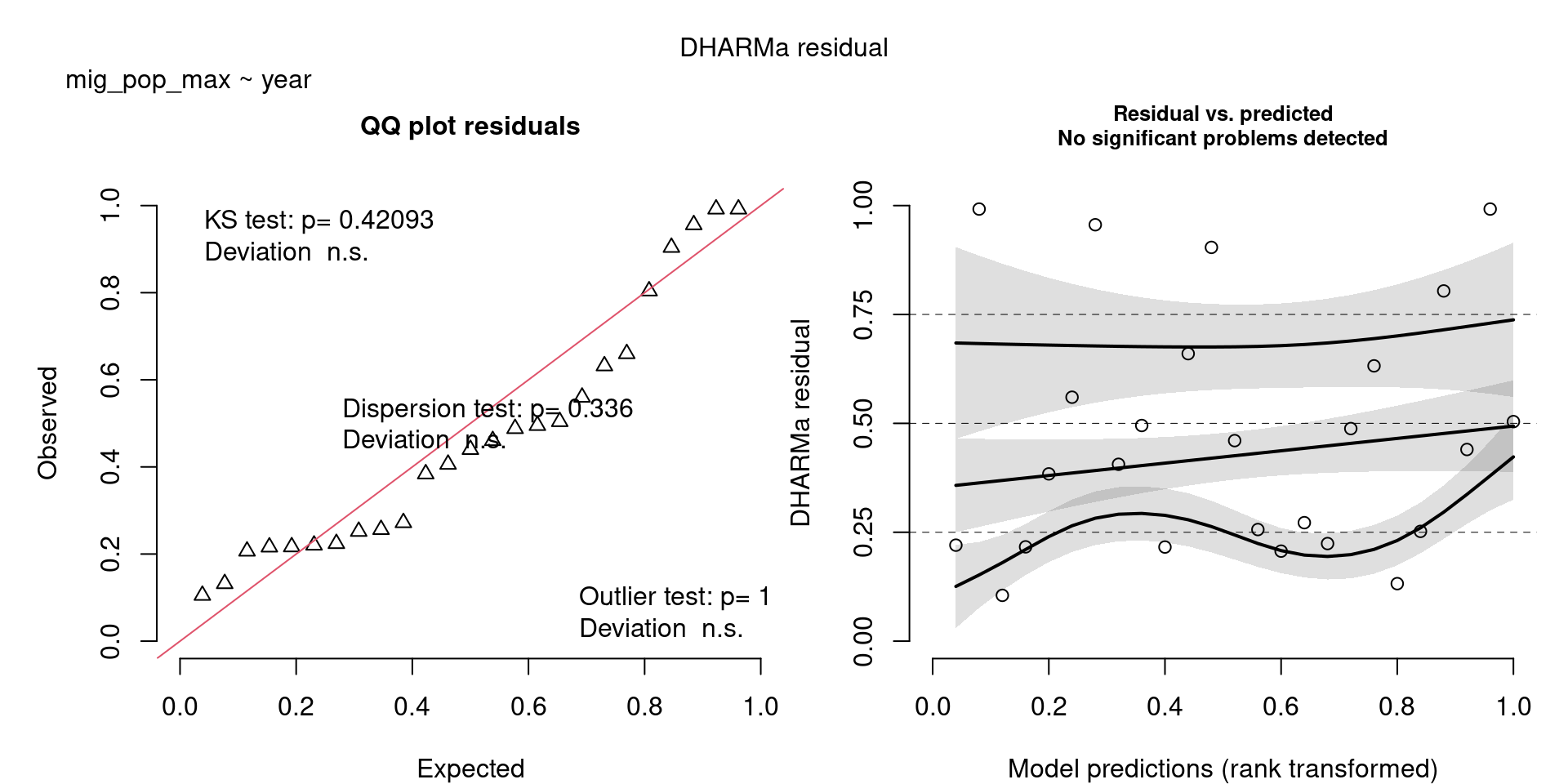
s <- simulateResiduals(x2, plot = TRUE)
title("log10 - mig_raw_max ~ year")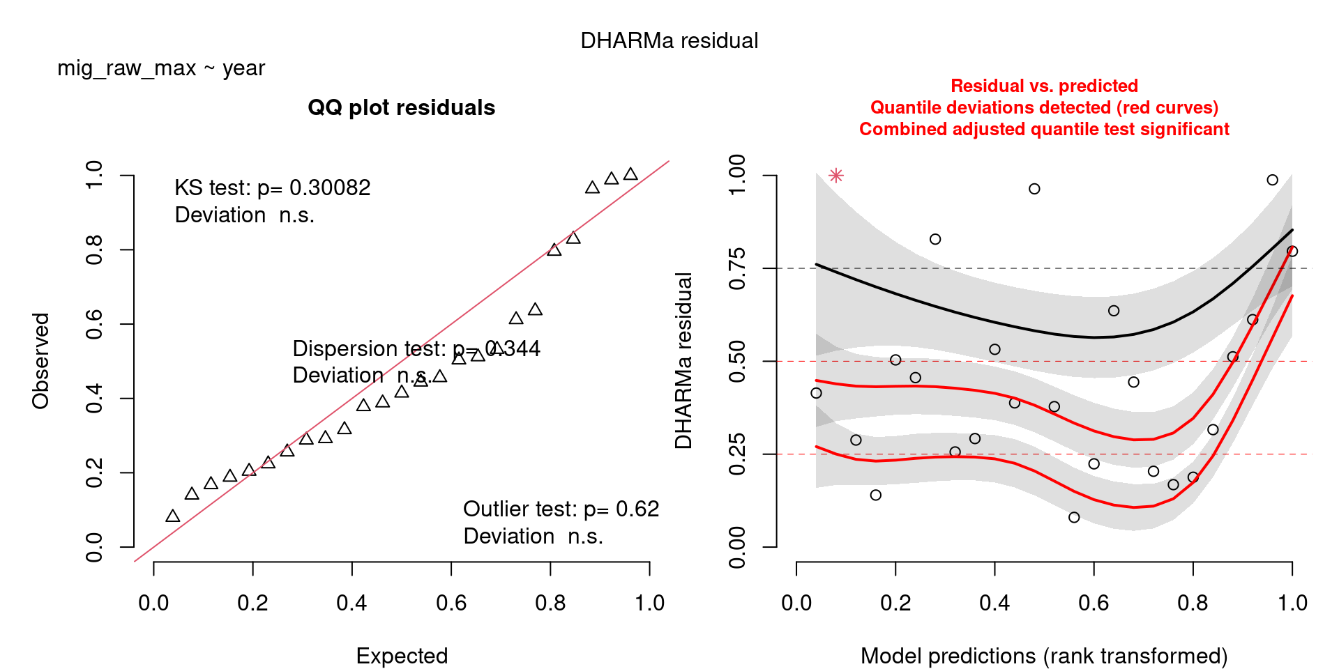
s <- simulateResiduals(y1, plot = TRUE)
title("Poisson - mig_pop_max ~ year")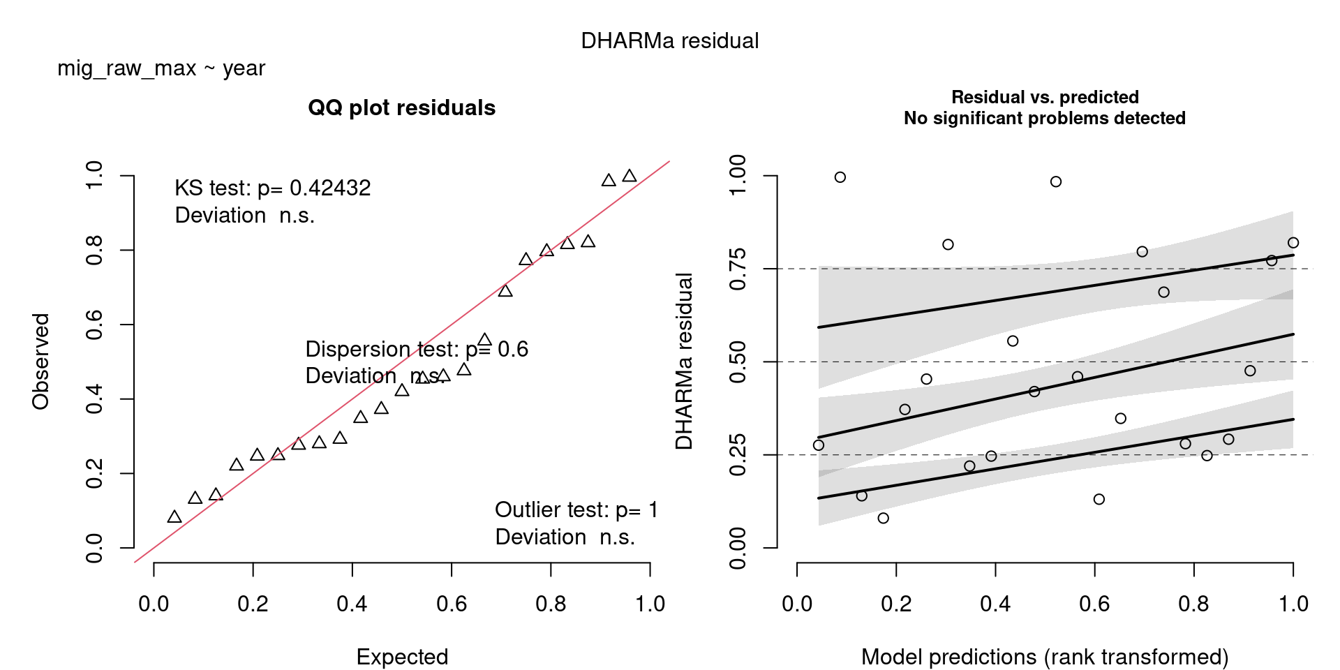
s <- simulateResiduals(y2, plot = TRUE)
title("Poisson - mig_raw_max ~ year")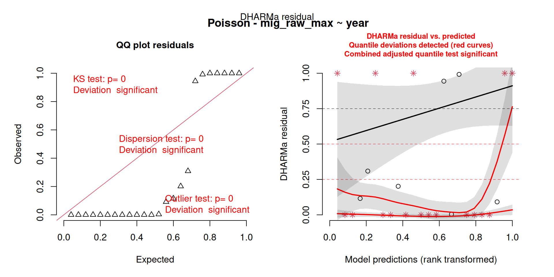
Tabulated Results
All the measures are significant. There was an increase in the maximum number of birds in kettles in both the raw counts as well as the predicted max.
Code
t <- get_table(models)
write_csv(filter(t, n != 23), "Data/Datasets/table_pop_mig.csv")
fmt_table(t)| term | estimate | estimate exp | std error | statistic | p value | n |
|---|---|---|---|---|---|---|
| mig_pop_max ~ year | ||||||
| (Intercept) | −61.797 | 0.000 | 21.547 | −2.868 | 0.004 | 24 |
| year | 0.034 | 1.034 | 0.011 | 3.149 | 0.002 | 24 |
| mig_raw_max ~ year | ||||||
| (Intercept) | −76.141 | 0.000 | 21.342 | −3.568 | 0.000 | 24 |
| year | 0.041 | 1.042 | 0.011 | 3.880 | 0.000 | 24 |
| (Intercept) | −45.812 | 0.000 | 21.627 | −2.118 | 0.034 | 22 |
| year | 0.026 | 1.026 | 0.011 | 2.422 | 0.015 | 22 |
Code
pop_figs <- v |>
  select(year, mig_pop_max, mig_raw_max) |>
  pivot_longer(-year, names_to = "measure", values_to = "pop")

ggplot(pop_figs, aes(x = year, y = pop, group = measure, colour = measure)) +
  theme_bw() +
  geom_point() +
  stat_smooth(method = MASS::glm.nb) +
  scale_colour_viridis_d(end = 0.8)
`geom_smooth()` using formula = 'y ~ x'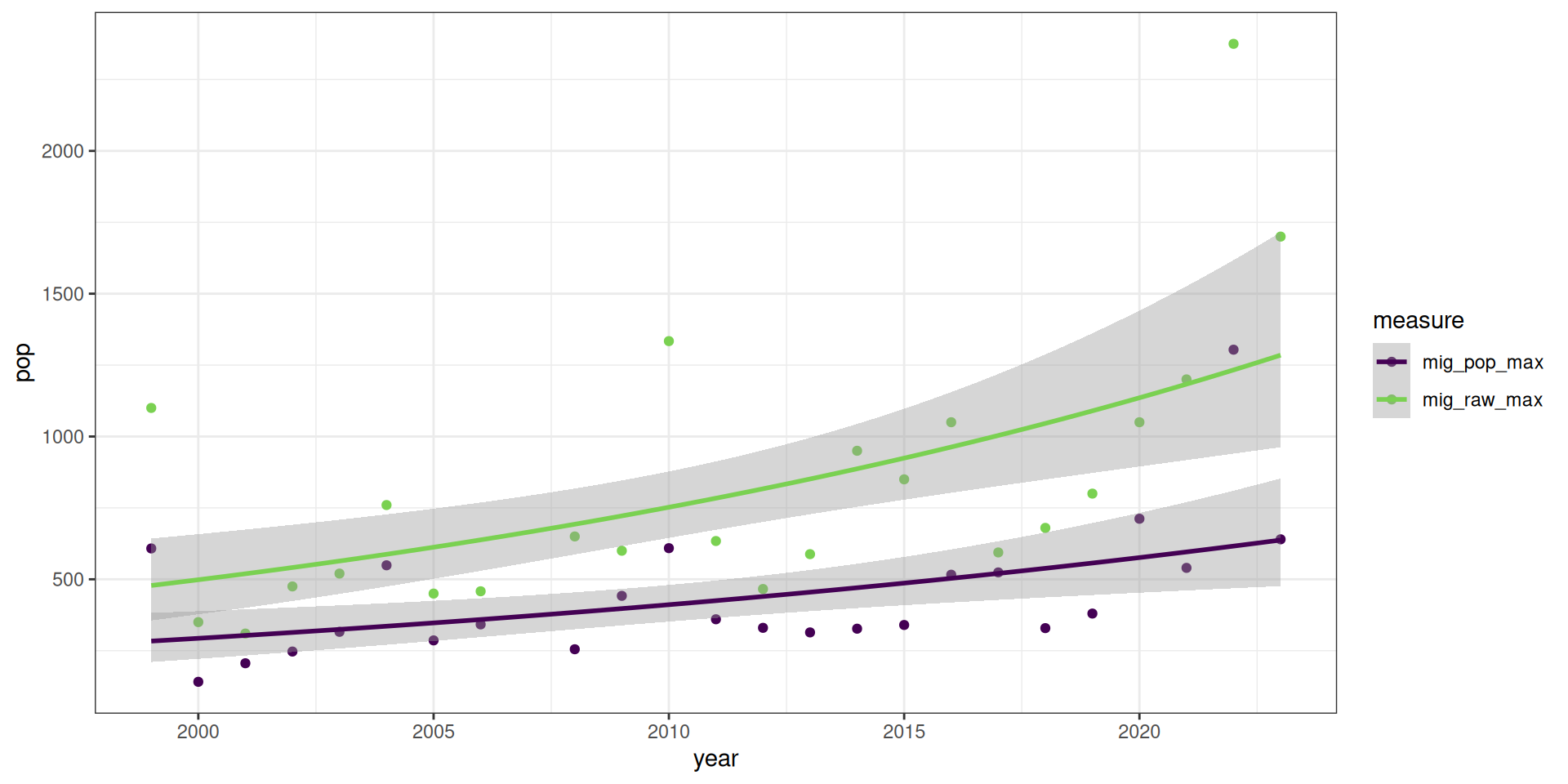
Code
model_check_figs(models)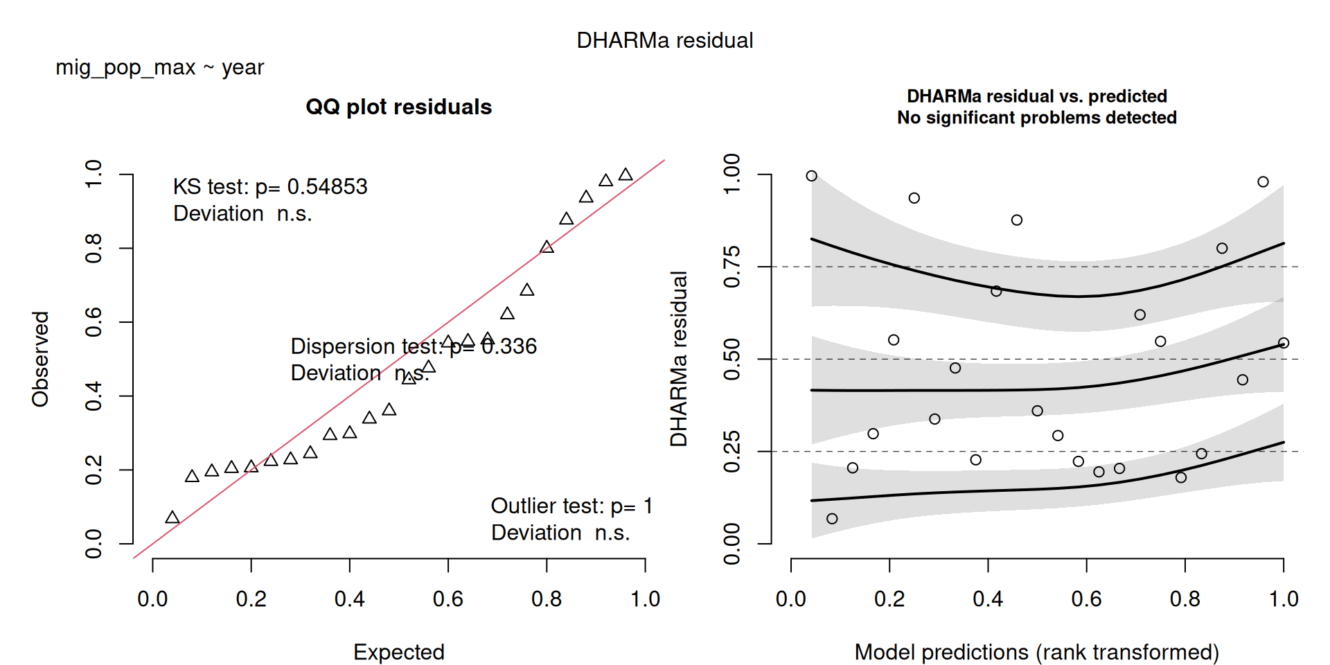
The DHARMa model checks don’t highlight any particular outlier problems, but out of an abundance of caution, we’ll do a quick review of any high Cook’s D values.
Values highlighted in red are more than 4/25, a standard Cook’s D cutoff (4/sample size). These indicate potential influential data points for a particular model.
Code
get_cooks(models[-3]) |>
gt_cooks()| Cook's Distances | ||
|---|---|---|
| year | mig_pop_max | mig_raw_max |
| 1999 | 0.97 | 1.28 |
| 2000 | 0.17 | 0.06 |
| 2001 | 0.06 | 0.09 |
| 2002 | 0.02 | 0.01 |
| 2003 | 0.00 | 0.00 |
| 2004 | 0.13 | 0.03 |
| 2005 | 0.01 | 0.02 |
| 2006 | 0.00 | 0.02 |
| 2008 | 0.02 | 0.00 |
| 2009 | 0.00 | 0.00 |
| 2010 | 0.04 | 0.10 |
| 2011 | 0.00 | 0.01 |
| 2012 | 0.01 | 0.03 |
| 2013 | 0.02 | 0.02 |
| 2014 | 0.02 | 0.00 |
| 2015 | 0.02 | 0.00 |
| 2016 | 0.00 | 0.00 |
| 2017 | 0.00 | 0.05 |
| 2018 | 0.05 | 0.04 |
| 2019 | 0.04 | 0.03 |
| 2020 | 0.02 | 0.00 |
| 2021 | 0.00 | 0.00 |
| 2022 | 0.76 | 0.53 |
| 2023 | 0.00 | 0.08 |
Check influential points
Now let’s see what happens if we were to omit these years from the respective analyses.
Tables with coefficients for both original and new model are shown, with colour intensity showing strength in the pattern.
For the maximum population recorded during migration based on both predicted counts and raw counts, if we omit 1999, the patterns are stronger, but the same.
compare(m1, 1999)| model | parameter | Estimate | Std. Error | z value | Pr(>|z|) |
|---|---|---|---|---|---|
| Original - mig_pop_max | (Intercept) | -61.797 | 21.547 | -2.868 | 0.004 |
| Drop 1999 - mig_pop_max | (Intercept) | -88.105 | 19.999 | -4.405 | 0.000 |
| Original - mig_pop_max | year | 0.034 | 0.011 | 3.149 | 0.002 |
| Drop 1999 - mig_pop_max | year | 0.047 | 0.010 | 4.707 | 0.000 |
compare(m2, 1999)| model | parameter | Estimate | Std. Error | z value | Pr(>|z|) |
|---|---|---|---|---|---|
| Original - mig_raw_max | (Intercept) | -76.141 | 21.342 | -3.568 | 0 |
| Drop 1999 - mig_raw_max | (Intercept) | -106.053 | 18.756 | -5.654 | 0 |
| Original - mig_raw_max | year | 0.041 | 0.011 | 3.880 | 0 |
| Drop 1999 - mig_raw_max | year | 0.056 | 0.009 | 6.008 | 0 |
If we omit 2000 or 2022, the patterns are weaker, but still the same.
compare(m1, 2000)| model | parameter | Estimate | Std. Error | z value | Pr(>|z|) |
|---|---|---|---|---|---|
| Original - mig_pop_max | (Intercept) | -61.797 | 21.547 | -2.868 | 0.004 |
| Drop 2000 - mig_pop_max | (Intercept) | -53.042 | 21.731 | -2.441 | 0.015 |
| Original - mig_pop_max | year | 0.034 | 0.011 | 3.149 | 0.002 |
| Drop 2000 - mig_pop_max | year | 0.029 | 0.011 | 2.721 | 0.006 |
compare(m1, 2022)| model | parameter | Estimate | Std. Error | z value | Pr(>|z|) |
|---|---|---|---|---|---|
| Original - mig_pop_max | (Intercept) | -61.797 | 21.547 | -2.868 | 0.004 |
| Drop 2022 - mig_pop_max | (Intercept) | -40.321 | 19.944 | -2.022 | 0.043 |
| Original - mig_pop_max | year | 0.034 | 0.011 | 3.149 | 0.002 |
| Drop 2022 - mig_pop_max | year | 0.023 | 0.010 | 2.322 | 0.020 |
compare(m2, 2022)| model | parameter | Estimate | Std. Error | z value | Pr(>|z|) |
|---|---|---|---|---|---|
| Original - mig_raw_max | (Intercept) | -76.141 | 21.342 | -3.568 | 0.000 |
| Drop 2022 - mig_raw_max | (Intercept) | -59.119 | 20.655 | -2.862 | 0.004 |
| Original - mig_raw_max | year | 0.041 | 0.011 | 3.880 | 0.000 |
| Drop 2022 - mig_raw_max | year | 0.033 | 0.010 | 3.182 | 0.001 |
In addition to the sensitivity check using cook’s distances, here we will conduct a more targeted exploration of some specific years.
Gaps around the peak
First, we consider removing 2011 and 2013 as they have sampling gaps around the peak of migration
y <- c(2011, 2013)
m1a <- update(m1, data = filter(v, !year %in% y))
m2a <- update(m2, data = filter(v, !year %in% y))
models_a <- list(m1a, m2a)
Comparing the summary tables shows only superficial differences.
Data saved to Data/Datasets/table_supplemental.csv
Original
fmt_summary(models[1:2], intercept = FALSE)
to <- get_table(models[1:2]) |>
  select(model, term, estimate, std_error, statistic, p_value) |>
  mutate(type = "original")
write_csv(to, d, append = TRUE)| model | Parameter | Estimate | Std. Error | Z | P |
|---|---|---|---|---|---|
| mig_pop_max ~ year | year | 0.034 | 0.011 | 3.149 | 0.002 |
| mig_raw_max ~ year | year | 0.041 | 0.011 | 3.880 | 0.000 |
Years removed
fmt_summary(models_a, intercept = FALSE)
ta <- get_table(models_a) |>
  select(model, term, estimate, std_error, statistic, p_value) |>
  mutate(type = "gaps_removed")
write_csv(ta, d, append = TRUE)| model | Parameter | Estimate | Std. Error | Z | P |
|---|---|---|---|---|---|
| mig_pop_max ~ year | year | 0.034 | 0.011 | 3.117 | 0.002 |
| mig_raw_max ~ year | year | 0.042 | 0.011 | 3.842 | 0.000 |
Missing the end of migration
Second, we consider removing 2001, 2006, 2023 as they were three years where it looks like sampling ended earlier than the end of migration.
y <- c(2001, 2006, 2023)
m1b <- update(m1, data = filter(v, !year %in% y))
m2b <- update(m2, data = filter(v, !year %in% y))
models_b <- list(m1b, m2b)
Comparing the summary tables shows only superficial differences.
Data saved to Data/Datasets/table_supplemental.csv
Original
fmt_summary(models[1:2], intercept = FALSE)| model | Parameter | Estimate | Std. Error | Z | P |
|---|---|---|---|---|---|
| mig_pop_max ~ year | year | 0.034 | 0.011 | 3.149 | 0.002 |
| mig_raw_max ~ year | year | 0.041 | 0.011 | 3.880 | 0.000 |
Years removed
fmt_summary(models_b, intercept = FALSE)
tb <- get_table(models_b) |>
  select(model, term, estimate, std_error, statistic, p_value) |>
  mutate(type = "end_removed")
write_csv(tb, d, append = TRUE)| model | Parameter | Estimate | Std. Error | Z | P |
|---|---|---|---|---|---|
| mig_pop_max ~ year | year | 0.031 | 0.013 | 2.439 | 0.015 |
| mig_raw_max ~ year | year | 0.033 | 0.012 | 2.811 | 0.005 |
Remove all problematic years
Out of curiosity, let’s try removing all 5 years. This reduces our data from 25 to 19 samples, so is a substantial change and we may see non-significant results merely because we have removed too many samples.
y <- c(2011, 2013, 2001, 2006, 2023)
m1c <- update(m1, data = filter(v, !year %in% y))
m2c <- update(m2, data = filter(v, !year %in% y))
models_c <- list(m1c, m2c)
Comparing the summary tables shows only superficial differences.
Data saved to Data/Datasets/table_supplemental.csv
Original
fmt_summary(models[1:2], intercept = FALSE)| model | Parameter | Estimate | Std. Error | Z | P |
|---|---|---|---|---|---|
| mig_pop_max ~ year | year | 0.034 | 0.011 | 3.149 | 0.002 |
| mig_raw_max ~ year | year | 0.041 | 0.011 | 3.880 | 0.000 |
Years removed
fmt_summary(models_c, intercept = FALSE)
tc <- get_table(models_c) |>
  select(model, term, estimate, std_error, statistic, p_value) |>
  mutate(type = "all_removed")
write_csv(tc, d, append = TRUE)| model | Parameter | Estimate | Std. Error | Z | P |
|---|---|---|---|---|---|
| mig_pop_max ~ year | year | 0.031 | 0.013 | 2.411 | 0.016 |
| mig_raw_max ~ year | year | 0.034 | 0.012 | 2.790 | 0.005 |
Conclusions
I do not believe that these potentially problematic sampling years are driving the patterns we see in this data.
Code
map(models, summary)[[1]]
Call:
MASS::glm.nb(formula = mig_pop_max ~ year, data = v, init.theta = 6.906339287,
link = log)
Coefficients:
Estimate Std. Error z value Pr(>|z|)
(Intercept) -61.79691 21.54677 -2.868 0.00413 **
year 0.03374 0.01071 3.149 0.00164 **
---
Signif. codes: 0 '***' 0.001 '**' 0.01 '*' 0.05 '.' 0.1 ' ' 1
(Dispersion parameter for Negative Binomial(6.9063) family taken to be 1)
Null deviance: 35.662 on 23 degrees of freedom
Residual deviance: 24.554 on 22 degrees of freedom
AIC: 316.49
Number of Fisher Scoring iterations: 1
Theta: 6.91
Std. Err.: 1.98
2 x log-likelihood: -310.494
[[2]]
Call:
MASS::glm.nb(formula = mig_raw_max ~ year, data = v, init.theta = 6.987056274,
link = log)
Coefficients:
Estimate Std. Error z value Pr(>|z|)
(Intercept) -76.14124 21.34238 -3.568 0.000360 ***
year 0.04118 0.01061 3.880 0.000104 ***
---
Signif. codes: 0 '***' 0.001 '**' 0.01 '*' 0.05 '.' 0.1 ' ' 1
(Dispersion parameter for Negative Binomial(6.9871) family taken to be 1)
Null deviance: 41.646 on 23 degrees of freedom
Residual deviance: 24.554 on 22 degrees of freedom
AIC: 345.5
Number of Fisher Scoring iterations: 1
Theta: 6.99
Std. Err.: 1.99
2 x log-likelihood: -339.505
[[3]]
Call:
MASS::glm.nb(formula = mig_raw_max ~ year, data = filter(v, mig_raw_max <
1500), init.theta = 8.726319225, link = log)
Coefficients:
Estimate Std. Error z value Pr(>|z|)
(Intercept) -45.81205 21.62744 -2.118 0.0342 *
year 0.02606 0.01076 2.422 0.0154 *
---
Signif. codes: 0 '***' 0.001 '**' 0.01 '*' 0.05 '.' 0.1 ' ' 1
(Dispersion parameter for Negative Binomial(8.7263) family taken to be 1)
Null deviance: 28.568 on 21 degrees of freedom
Residual deviance: 22.414 on 20 degrees of freedom
AIC: 308.17
Number of Fisher Scoring iterations: 1
Theta: 8.73
Std. Err.: 2.62
2 x log-likelihood: -302.166 Number of residents
How many resident vultures are there? Has this changed?
- Look for changes in the median number of residents
res_pop_median,res_raw_median
Descriptive stats
Code
v |>
  select("res_pop_median", "res_raw_median") |>
desc_stats()| measure | mean | sd | min | median | max | n |
|---|---|---|---|---|---|---|
| res_pop_median | 5.62 | 2.68 | 2 | 5.0 | 12 | 24 |
| res_raw_median | 4.96 | 2.14 | 1 | 4.5 | 8 | 24 |
m1 <- glm(res_pop_median ~ year, family = "poisson", data = v)
m2 <- glm(res_raw_median ~ year, family = "poisson", data = v)

models <- list(m1, m2)
Not used, but included for completeness
x1 <- lm(log10(res_pop_median) ~ year, data = v)
x2 <- lm(log10(res_raw_median) ~ year, data = v)

s <- simulateResiduals(x1, plot = TRUE)
Warning in newton(lsp = lsp, X = G$X, y = G$y, Eb = G$Eb, UrS = G$UrS, L = G$L,
: Fitting terminated with step failure - check results carefullytitle("log10 - res_pop_median ~ year")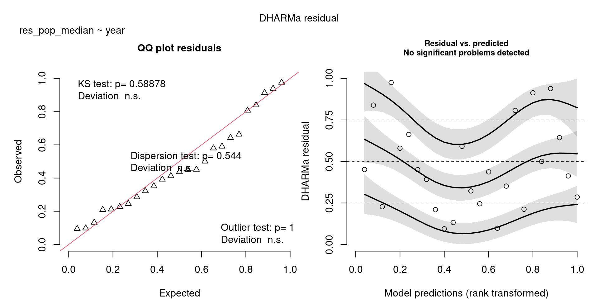
s <- simulateResiduals(x2, plot = TRUE)
title("log10 - res_raw_median ~ year")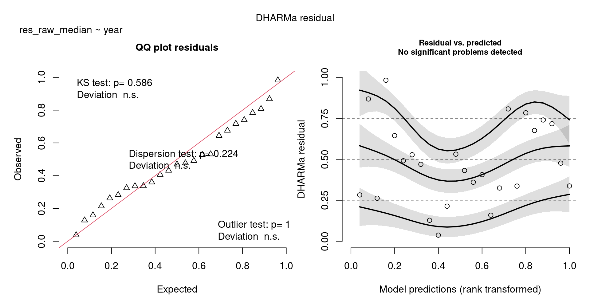
Tabulated Results
All measures are significant, there is an increase in the number of resident birds over the years.
Code
t <- get_table(models)
write_csv(t, "Data/Datasets/table_pop_res.csv")
fmt_table(t)| term | estimate | estimate exp | std error | statistic | p value | n |
|---|---|---|---|---|---|---|
| res_pop_median ~ year | ||||||
| (Intercept) | −79.712 | 0.000 | 24.549 | −3.247 | 0.001 | 24 |
| year | 0.040 | 1.041 | 0.012 | 3.319 | 0.001 | 24 |
| res_raw_median ~ year | ||||||
| (Intercept) | −60.538 | 0.000 | 25.804 | −2.346 | 0.019 | 24 |
| year | 0.031 | 1.031 | 0.013 | 2.409 | 0.016 | 24 |
Code
res_figs <- v |>
  select(year, res_pop_median, res_raw_median) |>
  pivot_longer(-year, names_to = "measure", values_to = "pop")

ggplot(res_figs, aes(x = year, y = pop, group = measure, colour = measure)) +
  theme_bw() +
  geom_point() +
  geom_smooth(method = "glm", method.args = list(family = "poisson")) +
  scale_colour_viridis_d(end = 0.8)
`geom_smooth()` using formula = 'y ~ x'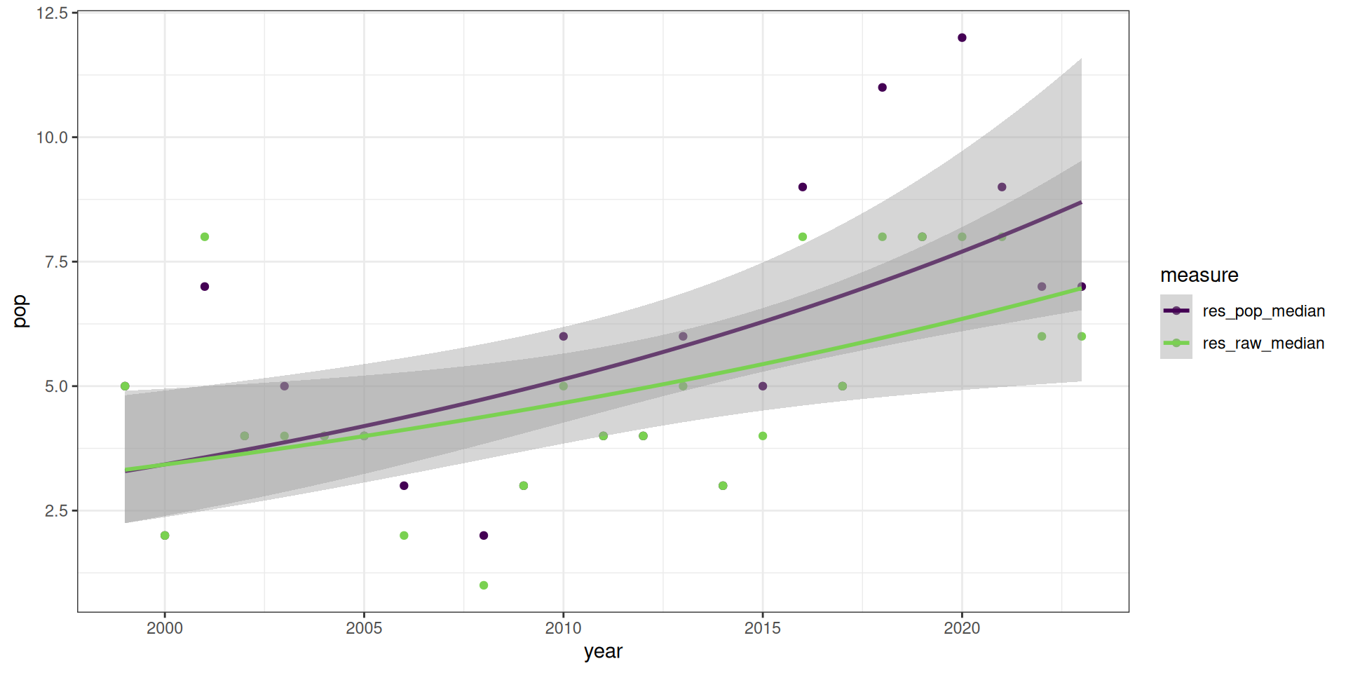
Code
model_check_figs(models)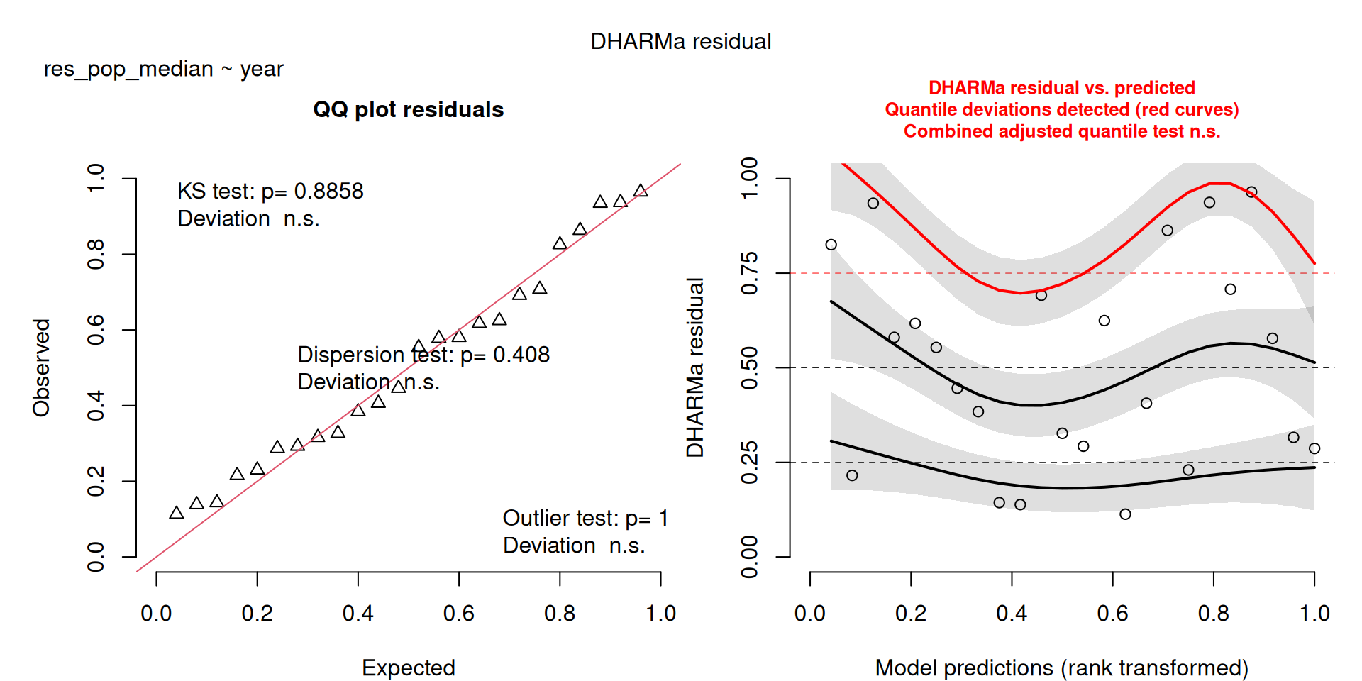
The DHARMa model checks don’t highlight any particular outlier problems, but out of an abundance of caution, we’ll do a quick review of any high Cook’s D values.
Values highlighted in red are more than 4/25, a standard Cook’s D cutoff (4/sample size). These indicate potential influential data points for a particular model.
Code
get_cooks(models) |>
gt_cooks()| Cook's Distances | ||
|---|---|---|
| year | res_pop_median | res_raw_median |
| 1999 | 0.07 | 0.07 |
| 2000 | 0.04 | 0.05 |
| 2001 | 0.22 | 0.39 |
| 2002 | 0.00 | 0.00 |
| 2003 | 0.02 | 0.00 |
| 2004 | 0.00 | 0.00 |
| 2005 | 0.00 | 0.00 |
| 2006 | 0.02 | 0.04 |
| 2008 | 0.05 | 0.08 |
| 2009 | 0.02 | 0.01 |
| 2010 | 0.00 | 0.00 |
| 2011 | 0.01 | 0.00 |
| 2012 | 0.01 | 0.00 |
| 2013 | 0.00 | 0.00 |
| 2014 | 0.04 | 0.02 |
| 2015 | 0.01 | 0.01 |
| 2016 | 0.03 | 0.03 |
| 2017 | 0.02 | 0.00 |
| 2018 | 0.10 | 0.03 |
| 2019 | 0.00 | 0.03 |
| 2020 | 0.16 | 0.03 |
| 2021 | 0.01 | 0.03 |
| 2022 | 0.02 | 0.01 |
| 2023 | 0.05 | 0.02 |
Check influential points
Now let’s see what happens if we were to omit these years from the respective analyses.
Tables with coefficients for both original and new model are shown, with colour intensity showing strength in the pattern.
For the daily median number of resident birds based on both predicted counts and raw counts, if we omit 2001, the patterns are stronger, but the same.
compare(m1, 2001)| model | parameter | Estimate | Std. Error | z value | Pr(>|z|) |
|---|---|---|---|---|---|
| Original - res_pop_median | (Intercept) | -79.712 | 24.549 | -3.247 | 0.001 |
| Drop 2001 - res_pop_median | (Intercept) | -94.397 | 26.293 | -3.590 | 0.000 |
| Original - res_pop_median | year | 0.040 | 0.012 | 3.319 | 0.001 |
| Drop 2001 - res_pop_median | year | 0.048 | 0.013 | 3.658 | 0.000 |
compare(m2, 2001)| model | parameter | Estimate | Std. Error | z value | Pr(>|z|) |
|---|---|---|---|---|---|
| Original - res_raw_median | (Intercept) | -60.538 | 25.804 | -2.346 | 0.019 |
| Drop 2001 - res_raw_median | (Intercept) | -81.261 | 27.918 | -2.911 | 0.004 |
| Original - res_raw_median | year | 0.031 | 0.013 | 2.409 | 0.016 |
| Drop 2001 - res_raw_median | year | 0.041 | 0.014 | 2.969 | 0.003 |
Code
map(models, summary)[[1]]
Call:
glm(formula = res_pop_median ~ year, family = "poisson", data = v)
Coefficients:
Estimate Std. Error z value Pr(>|z|)
(Intercept) -79.71246 24.54876 -3.247 0.001166 **
year 0.04047 0.01219 3.319 0.000903 ***
---
Signif. codes: 0 '***' 0.001 '**' 0.01 '*' 0.05 '.' 0.1 ' ' 1
(Dispersion parameter for poisson family taken to be 1)
Null deviance: 28.293 on 23 degrees of freedom
Residual deviance: 16.914 on 22 degrees of freedom
AIC: 104.74
Number of Fisher Scoring iterations: 4
[[2]]
Call:
glm(formula = res_raw_median ~ year, family = "poisson", data = v)
Coefficients:
Estimate Std. Error z value Pr(>|z|)
(Intercept) -60.53757 25.80385 -2.346 0.019 *
year 0.03088 0.01282 2.409 0.016 *
---
Signif. codes: 0 '***' 0.001 '**' 0.01 '*' 0.05 '.' 0.1 ' ' 1
(Dispersion parameter for poisson family taken to be 1)
Null deviance: 22.313 on 23 degrees of freedom
Residual deviance: 16.391 on 22 degrees of freedom
AIC: 101.33
Number of Fisher Scoring iterations: 4Patterns of migration
Is the timing of migration skewed to earlier or later in the season? Is this distribution of migration flattened and wide (low kurtosis) or peaked (high kurtosis) Are these patterns consistent over the years?
Kurtosis can be used to indicates if all the birds pass through in a relatively quick ‘clump’ (thick-tailed, lower kurtosis), or whether the migration stretches out over a longer period of time (long-tailed, higher kurtosis). Possible implications for conservation or future survey designs?
- Look for significant skew and kurtosis in migration (5-95%) and peak migration (25-75%)
mig_skew,peak_skew,mig_kurt,peak_kurt
Descriptive stats
Code
v |>
  select(contains("skew"), contains("kurt")) |>
desc_stats()| measure | mean | sd | min | median | max | n |
|---|---|---|---|---|---|---|
| mig_skew | 0.00 | 0.21 | -0.4442868 | -0.03392198 | 0.5067799 | 24 |
| peak_skew | 0.00 | 0.09 | -0.1296424 | -0.02295204 | 0.2880288 | 24 |
| all_skew | −0.06 | 0.20 | -0.4654119 | -0.05317408 | 0.3816406 | 24 |
| mig_kurt | −0.67 | 0.17 | -0.9329652 | -0.71138435 | -0.1280714 | 24 |
| peak_kurt | −1.12 | 0.03 | -1.1883554 | -1.12398983 | -1.0337500 | 24 |
| all_kurt | 0.27 | 0.58 | -0.3319748 | 0.20767601 | 2.5554292 | 24 |
Here we look at skew and excess kurtosis only against the intercept. This allows us to test for differences from 0.
- Skew of 0 is normal, but below or above are considered left- and right-skewed
- A normal distribution has an excess kurtosis of 0.
m1 <- lm(mig_skew ~ 1, data = v)
m2 <- lm(peak_skew ~ 1, data = v)
m3 <- lm(all_skew ~ 1, data = v)
m4 <- lm(mig_kurt ~ 1, data = v)
m5 <- lm(peak_kurt ~ 1, data = v)
m6 <- lm(all_kurt ~ 1, data = v)

models <- list(m1, m2, m3, m4, m5, m6)
Tabulated Results
Skew is not significantly different from zero in any period.
Kurtosis is significantly different from zero in all periods.
In the migration and peak migration periods, Kurtosis is negative, corresponding to thick-tailed distributions, squat distributions (closer to a uniform distribution).
However, in the ‘all’ period, kurtosis is actually significantly positive, corresponding to relatively more narrow, thin-tailed distributions.
Code
t <- get_table(models)
write_csv(t, "Data/Datasets/table_skew.csv")
fmt_table(t)| term | estimate | std error | statistic | p value | n |
|---|---|---|---|---|---|
| mig_skew ~ 1 (R2 = 0; R2-adj = 0) | |||||
| (Intercept) | −0.003 | 0.042 | −0.067 | 0.947 | 24 |
| peak_skew ~ 1 (R2 = 0; R2-adj = 0) | |||||
| (Intercept) | −0.003 | 0.018 | −0.166 | 0.869 | 24 |
| all_skew ~ 1 (R2 = 0; R2-adj = 0) | |||||
| (Intercept) | −0.063 | 0.041 | −1.531 | 0.139 | 24 |
| mig_kurt ~ 1 (R2 = 0; R2-adj = 0) | |||||
| (Intercept) | −0.674 | 0.034 | −19.567 | 0.000 | 24 |
| peak_kurt ~ 1 (R2 = 0; R2-adj = 0) | |||||
| (Intercept) | −1.124 | 0.006 | −174.493 | 0.000 | 24 |
| all_kurt ~ 1 (R2 = 0; R2-adj = 0) | |||||
| (Intercept) | 0.267 | 0.119 | 2.246 | 0.035 | 24 |
The periods
The “all” period is defined individually as being the dates centred on the date at the 50% percentile passage is reached and includes all dates from this date to the end of the year, and that same number of dates prior to the p50 date. See the Skewness & Kurtosis section in the last report.
By definition, the migration period (5-95%) and the peak migration period (25-75%) are truncated distributions, so I don’t think we can really interpret kurtosis for these subsets. With the “all” period, I have attempted to subset the data to get a good measure of the migration period only, but honestly, kurtosis depends so much on where I define the cutoffs I’m not really sure that we can accurately measure it. Looking at the figures, I’d say they’re narrower than normal (so positive kurtosis, which does align with the stats for the “all” period), but that’s just a visual estimate.
This is figure showing the statistics.
Code
dist_figs <- v |>
  select(year, contains("skew"), contains("kurt")) |>
  pivot_longer(cols = -year, names_to = "measure", values_to = "statistic")

ggplot(filter(dist_figs, year != 2001), aes(x = statistic, y = measure, fill = measure)) +
  theme_bw() +
  geom_vline(xintercept = 0, colour = "grey20", linetype = "dotted") +
  geom_boxplot() +
  scale_fill_viridis_d()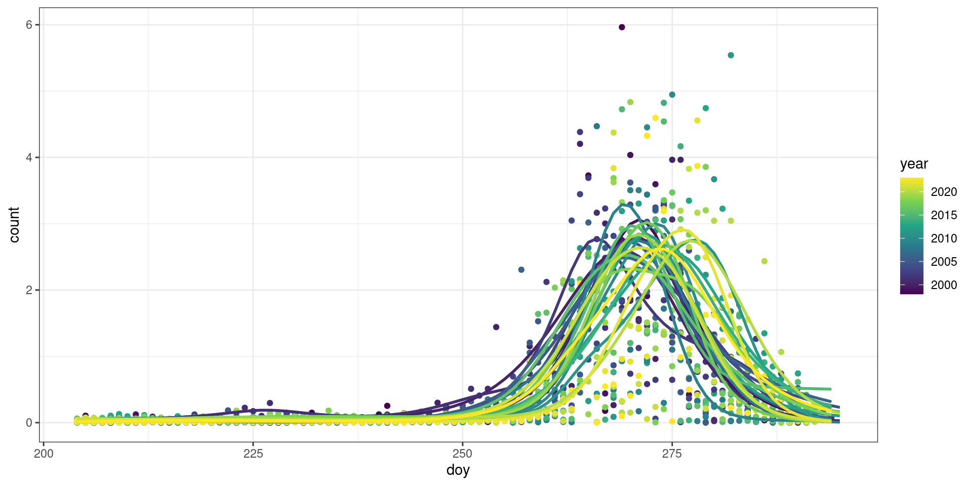
This figure shows the distributions in each year over top a normal distribution, for illustration.
I think this shows positive kurtosis. The black lines are simulated normal distributions simulated using the mean, SD and counts from the data.
Code
normal <- v |>
  select(year, max_doy, mig_pop_total) |>
  left_join(summarize(filter(pred, doy > 240), sd = sd(rep(doy, round(count))), .by = "year"),
            by = "year") |>
  mutate(doy = pmap(list(max_doy, sd, mig_pop_total),
                    \(x, y, z) as.integer(rnorm(mean = x, sd = y, n = z)))) |>
  unnest(doy) |>
  count(year, doy, name = "count")

ggplot(raw, aes(x = doy, y = count)) +
  theme_bw() +
  geom_smooth(data = normal, method = "gam", colour = "black", linewidth = 1.5) +
  geom_point(size = 1, aes(colour = year), na.rm = TRUE) +
  geom_line(data = pred, linewidth = 1, aes(group = year, colour = year), na.rm = TRUE) +
  scale_colour_viridis_c() +
  facet_wrap(~year, scales = "free")
`geom_smooth()` using formula = 'y ~ s(x, bs = "cs")'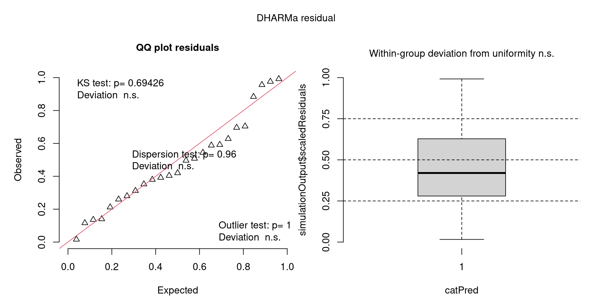
Here is a scaled view (counts are divided by the yearly standard deviation) of the patterns of migration using our GAM models from the “Calculate Metrics” step.
Code
raw_scaled <- raw |>
  mutate(across(c(count), \(x) scale(x, center = FALSE)),
         .by = "year")

pred_scaled <- pred |>
  mutate(across(c(count, ci99_upper, ci99_lower), \(x) scale(x, center = FALSE)),
         .by = "year")

ggplot(raw_scaled, aes(x = doy, y = count)) +
  theme_bw() +
  geom_point(aes(colour = year), na.rm = TRUE) +
  geom_line(data = pred_scaled, aes(colour = year, group = year),
            size = 1, na.rm = TRUE) +
  scale_colour_viridis_c()
Warning: Using `size` aesthetic for lines was deprecated in ggplot2 3.4.0.
ℹ Please use `linewidth` instead.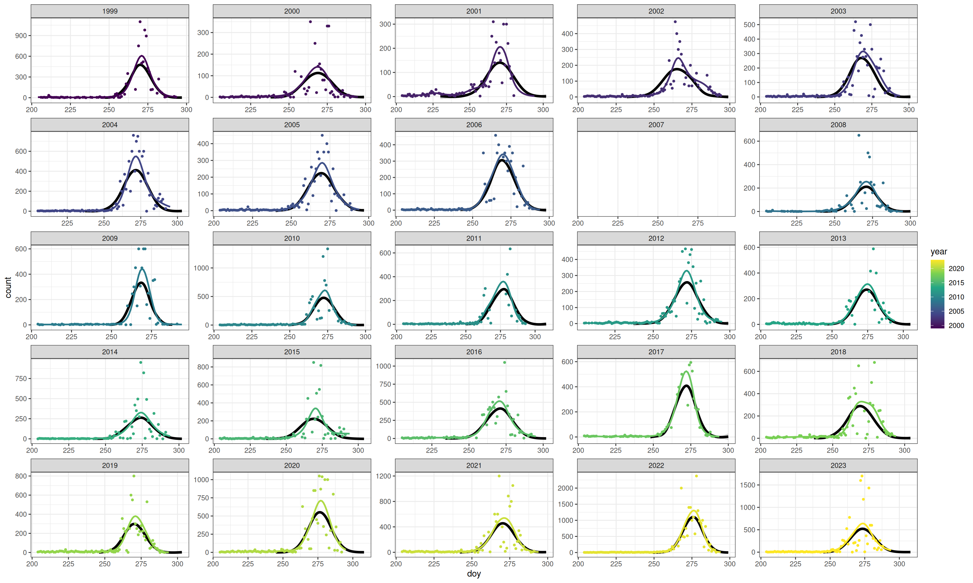
Code
model_check_figs(models)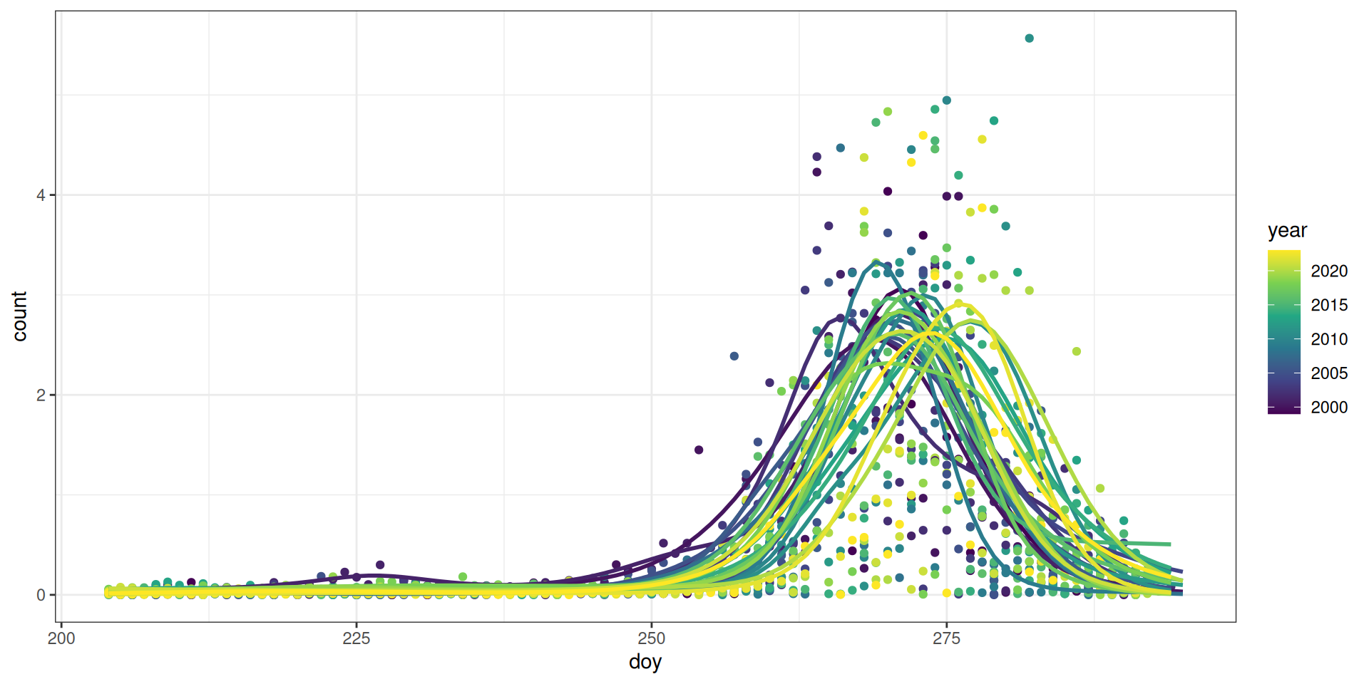

The DHARMa model checks don’t highlight any particular outlier problems, but out of an abundance of caution, we’ll do a quick review of any high Cook’s D values.
Values highlighted in red are more than 4/25, a standard Cook’s D cutoff (4/sample size). These indicate potential influential data points for a particular model.
Code
get_cooks(models) |>
gt_cooks()| Cook's Distances | ||||||
|---|---|---|---|---|---|---|
| year | mig_skew ~ 1 | peak_skew ~ 1 | all_skew ~ 1 | mig_kurt ~ 1 | peak_kurt ~ 1 | all_kurt ~ 1 |
| 1999 | 0.01 | 0.00 | 0.01 | 0.00 | 0.00 | 0.04 |
| 2000 | 0.02 | 0.03 | 0.02 | 0.00 | 0.00 | 0.00 |
| 2001 | 0.21 | 0.05 | 0.18 | 0.17 | 0.00 | 0.00 |
| 2002 | 0.16 | 0.47 | 0.05 | 0.00 | 0.37 | 0.01 |
| 2003 | 0.02 | 0.05 | 0.02 | 0.03 | 0.03 | 0.01 |
| 2004 | 0.15 | 0.09 | 0.21 | 0.09 | 0.08 | 0.00 |
| 2005 | 0.00 | 0.00 | 0.00 | 0.00 | 0.01 | 0.00 |
| 2006 | 0.00 | 0.00 | 0.00 | 0.03 | 0.00 | 0.02 |
| 2008 | 0.05 | 0.02 | 0.09 | 0.00 | 0.00 | 0.00 |
| 2009 | 0.00 | 0.00 | 0.02 | 0.00 | 0.08 | 0.70 |
| 2010 | 0.00 | 0.04 | 0.01 | 0.01 | 0.01 | 0.01 |
| 2011 | 0.04 | 0.09 | 0.01 | 0.02 | 0.00 | 0.05 |
| 2012 | 0.00 | 0.00 | 0.01 | 0.01 | 0.00 | 0.00 |
| 2013 | 0.00 | 0.00 | 0.00 | 0.02 | 0.00 | 0.04 |
| 2014 | 0.00 | 0.00 | 0.00 | 0.00 | 0.03 | 0.03 |
| 2015 | 0.28 | 0.10 | 0.22 | 0.47 | 0.13 | 0.00 |
| 2016 | 0.02 | 0.00 | 0.03 | 0.00 | 0.00 | 0.00 |
| 2017 | 0.03 | 0.03 | 0.05 | 0.00 | 0.00 | 0.03 |
| 2018 | 0.00 | 0.01 | 0.01 | 0.11 | 0.19 | 0.04 |
| 2019 | 0.01 | 0.01 | 0.04 | 0.03 | 0.01 | 0.01 |
| 2020 | 0.01 | 0.01 | 0.00 | 0.00 | 0.01 | 0.03 |
| 2021 | 0.02 | 0.01 | 0.02 | 0.02 | 0.07 | 0.00 |
| 2022 | 0.01 | 0.03 | 0.02 | 0.01 | 0.04 | 0.00 |
| 2023 | 0.00 | 0.01 | 0.00 | 0.00 | 0.00 | 0.02 |
Check influential points
Now let’s see what happens if we were to omit these years from the respective analyses.
Tables with coefficients for both original and new model are shown, with colour intensity showing strength in the pattern.
For 2001, the patterns shift but do not change.
compare(m1, 2001)| model | parameter | Estimate | Std. Error | t value | Pr(>|t|) |
|---|---|---|---|---|---|
| Original - mig_skew ~ 1 | (Intercept) | -0.003 | 0.042 | -0.067 | 0.947 |
| Drop 2001 - mig_skew ~ 1 | (Intercept) | 0.016 | 0.039 | 0.418 | 0.680 |
compare(m3, 2001)| model | parameter | Estimate | Std. Error | t value | Pr(>|t|) |
|---|---|---|---|---|---|
| Original - all_skew ~ 1 | (Intercept) | -0.063 | 0.041 | -1.531 | 0.139 |
| Drop 2001 - all_skew ~ 1 | (Intercept) | -0.045 | 0.039 | -1.169 | 0.255 |
compare(m4, 2001)| model | parameter | Estimate | Std. Error | t value | Pr(>|t|) |
|---|---|---|---|---|---|
| Original - mig_kurt ~ 1 | (Intercept) | -0.674 | 0.034 | -19.567 | 0 |
| Drop 2001 - mig_kurt ~ 1 | (Intercept) | -0.688 | 0.033 | -21.016 | 0 |
For 2002, the patterns are stronger.
compare(m2, 2002)| model | parameter | Estimate | Std. Error | t value | Pr(>|t|) |
|---|---|---|---|---|---|
| Original - peak_skew ~ 1 | (Intercept) | -0.003 | 0.018 | -0.166 | 0.869 |
| Drop 2002 - peak_skew ~ 1 | (Intercept) | -0.016 | 0.014 | -1.121 | 0.275 |
compare(m5, 2002)| model | parameter | Estimate | Std. Error | t value | Pr(>|t|) |
|---|---|---|---|---|---|
| Original - peak_kurt ~ 1 | (Intercept) | -1.124 | 0.006 | -174.493 | 0 |
| Drop 2002 - peak_kurt ~ 1 | (Intercept) | -1.128 | 0.005 | -211.632 | 0 |
For skew of the counts during the “all” period, if we omit 2004, the patterns are stronger, and nearly show a trend, but are still non-significant.
compare(m3, 2004)| model | parameter | Estimate | Std. Error | t value | Pr(>|t|) |
|---|---|---|---|---|---|
| Original - all_skew ~ 1 | (Intercept) | -0.063 | 0.041 | -1.531 | 0.139 |
| Drop 2004 - all_skew ~ 1 | (Intercept) | -0.082 | 0.038 | -2.147 | 0.043 |
For kurtosis during the “all” migration period, if we omit 2009, the patterns are less strong, but the same.
compare(m6, 2009)| model | parameter | Estimate | Std. Error | t value | Pr(>|t|) |
|---|---|---|---|---|---|
| Original - all_kurt ~ 1 | (Intercept) | 0.267 | 0.119 | 2.246 | 0.035 |
| Drop 2009 - all_kurt ~ 1 | (Intercept) | 0.167 | 0.068 | 2.467 | 0.022 |
For 2015, the patterns are stronger, but the same (i.e., not significant).
compare(m1, 2015)| model | parameter | Estimate | Std. Error | t value | Pr(>|t|) |
|---|---|---|---|---|---|
| Original - mig_skew ~ 1 | (Intercept) | -0.003 | 0.042 | -0.067 | 0.947 |
| Drop 2015 - mig_skew ~ 1 | (Intercept) | -0.025 | 0.037 | -0.667 | 0.512 |
compare(m3, 2015)| model | parameter | Estimate | Std. Error | t value | Pr(>|t|) |
|---|---|---|---|---|---|
| Original - all_skew ~ 1 | (Intercept) | -0.063 | 0.041 | -1.531 | 0.139 |
| Drop 2015 - all_skew ~ 1 | (Intercept) | -0.082 | 0.038 | -2.172 | 0.041 |
compare(m4, 2015)| model | parameter | Estimate | Std. Error | t value | Pr(>|t|) |
|---|---|---|---|---|---|
| Original - mig_kurt ~ 1 | (Intercept) | -0.674 | 0.034 | -19.567 | 0 |
| Drop 2015 - mig_kurt ~ 1 | (Intercept) | -0.697 | 0.026 | -26.758 | 0 |
For kurtosis during the peak migration period, if we omit 2018, the patterns don’t really change.
compare(m5, 2018)| model | parameter | Estimate | Std. Error | t value | Pr(>|t|) |
|---|---|---|---|---|---|
| Original - peak_kurt ~ 1 | (Intercept) | -1.124 | 0.006 | -174.493 | 0 |
| Drop 2018 - peak_kurt ~ 1 | (Intercept) | -1.121 | 0.006 | -184.887 | 0 |
Code
map(models, summary)[[1]]
Call:
lm(formula = mig_skew ~ 1, data = v)
Residuals:
Min 1Q Median 3Q Max
-0.44147 -0.11385 -0.03111 0.07105 0.50959
Coefficients:
Estimate Std. Error t value Pr(>|t|)
(Intercept) -0.002813 0.042126 -0.067 0.947
Residual standard error: 0.2064 on 23 degrees of freedom
[[2]]
Call:
lm(formula = peak_skew ~ 1, data = v)
Residuals:
Min 1Q Median 3Q Max
-0.12657 -0.06225 -0.01988 0.02682 0.29110
Coefficients:
Estimate Std. Error t value Pr(>|t|)
(Intercept) -0.003073 0.018460 -0.166 0.869
Residual standard error: 0.09044 on 23 degrees of freedom
[[3]]
Call:
lm(formula = all_skew ~ 1, data = v)
Residuals:
Min 1Q Median 3Q Max
-0.40252 -0.13270 0.00971 0.08692 0.44453
Coefficients:
Estimate Std. Error t value Pr(>|t|)
(Intercept) -0.06289 0.04108 -1.531 0.139
Residual standard error: 0.2012 on 23 degrees of freedom
[[4]]
Call:
lm(formula = mig_kurt ~ 1, data = v)
Residuals:
Min 1Q Median 3Q Max
-0.25928 -0.10693 -0.03770 0.04197 0.54561
Coefficients:
Estimate Std. Error t value Pr(>|t|)
(Intercept) -0.67368 0.03443 -19.57 7.79e-16 ***
---
Signif. codes: 0 '***' 0.001 '**' 0.01 '*' 0.05 '.' 0.1 ' ' 1
Residual standard error: 0.1687 on 23 degrees of freedom
[[5]]
Call:
lm(formula = peak_kurt ~ 1, data = v)
Residuals:
Min 1Q Median 3Q Max
-0.064172 -0.013194 0.000194 0.006965 0.090433
Coefficients:
Estimate Std. Error t value Pr(>|t|)
(Intercept) -1.124183 0.006443 -174.5 <2e-16 ***
---
Signif. codes: 0 '***' 0.001 '**' 0.01 '*' 0.05 '.' 0.1 ' ' 1
Residual standard error: 0.03156 on 23 degrees of freedom
[[6]]
Call:
lm(formula = all_kurt ~ 1, data = v)
Residuals:
Min 1Q Median 3Q Max
-0.59881 -0.36626 -0.05916 0.15063 2.28859
Coefficients:
Estimate Std. Error t value Pr(>|t|)
(Intercept) 0.2668 0.1188 2.246 0.0346 *
---
Signif. codes: 0 '***' 0.001 '**' 0.01 '*' 0.05 '.' 0.1 ' ' 1
Residual standard error: 0.5821 on 23 degrees of freedom