source("XX_functions.R")  # Custom functions and packages

set.seed(1234) # To make this reproducible

v <- read_csv("Data/Datasets/vultures_clean_2023.csv")
resident_date <- 240Calculate Metrics
Background
Having explored the data (Initial Exploration) and various ways of calculating metrics of migration timing, we will now calculate and explore these metrics for the entire data set.
We will use
- a GAM approach to model the pattern of vulture counts
- percentiles based on cumulative modelled counts to assess dates of passage
- Option 3 to account for resident birds (subtract the predicted mean residents prior to calculating the cumulative counts)
Load Data
Metrics to assess
To answer these questions we will summarize the counts into specific metrics representing the timing of migration.
Specifically, we would like to calculate the
- dates of 5%, 25%, 50%, 75%, and 95% of the kettle numbers
- duration of passage - No. days between 5% and 95%
- duration of peak passage - No. days between 25% and 75%
Population size (no. vultures in aggregations)
- maximum
- cumulative
- number at peak passage (mean, median, range)
- number of locals (mean, median, range)
Of these, the most important starting metrics are the dates of 5%, 25%, 50%, 75%, and 95% of the kettle numbers. These dates will define migration phenology as well as local vs. migrating counts. All other calculations can be performed using these values and the raw data.
Proceedure
The steps for calculating these metrics are as follows.
For each year we will calculate…
- A GAM
- The median number of residents, using day 240 as a cutoff
- The cumulative migration counts
- The dates of passage as percentiles of these cumulative counts (5%, 25%, 75%, 95%)
- The duration of (peak) passage from these dates
- The population size (max, cumulative, stats at peak passage, stats of locals)
We will also create figures outlining these metrics for each year and will use these to assess whether anything needs to be tweaked (i.e. perhaps the date 240 cutoff)
Calculate Metrics
0. Sample sizes
samples <- v |>
  group_by(year) |>
  filter(!is.na(count)) |> # Omit missing dates
  summarize(
    date_min = min(date), date_max = max(date),
    # number of dates with a count
    n_dates_obs = n(),
    # number of dates in the range
    n_dates = as.numeric(difftime(date_max, date_min, units = "days")),
n_obs = sum(count))gt(samples)| year | date_min | date_max | n_dates_obs | n_dates | n_obs |
|---|---|---|---|---|---|
| 1999 | 1999-07-25 | 1999-10-20 | 64 | 87 | 7397 |
| 2000 | 2000-07-23 | 2000-10-18 | 76 | 87 | 2623 |
| 2001 | 2001-07-23 | 2001-10-07 | 64 | 76 | 3366 |
| 2002 | 2002-07-23 | 2002-10-21 | 83 | 90 | 4454 |
| 2003 | 2003-07-23 | 2003-10-18 | 83 | 87 | 6229 |
| 2004 | 2004-07-23 | 2004-10-18 | 80 | 87 | 9052 |
| 2005 | 2005-07-23 | 2005-10-18 | 83 | 87 | 5267 |
| 2006 | 2006-07-23 | 2006-10-17 | 73 | 86 | 5317 |
| 2008 | 2008-07-23 | 2008-10-17 | 59 | 86 | 3761 |
| 2009 | 2009-07-23 | 2009-10-18 | 62 | 87 | 5257 |
| 2010 | 2010-07-23 | 2010-10-18 | 75 | 87 | 7956 |
| 2011 | 2011-07-24 | 2011-10-20 | 69 | 88 | 3032 |
| 2012 | 2012-07-23 | 2012-10-18 | 78 | 87 | 5327 |
| 2013 | 2013-07-23 | 2013-10-18 | 69 | 87 | 4006 |
| 2014 | 2014-07-23 | 2014-10-18 | 74 | 87 | 6021 |
| 2015 | 2015-07-23 | 2015-10-18 | 77 | 87 | 5428 |
| 2016 | 2016-07-23 | 2016-10-18 | 68 | 87 | 8137 |
| 2017 | 2017-07-23 | 2017-10-17 | 62 | 86 | 4827 |
| 2018 | 2018-07-23 | 2018-10-18 | 75 | 87 | 6672 |
| 2019 | 2019-07-23 | 2019-10-18 | 87 | 87 | 6476 |
| 2020 | 2020-07-23 | 2020-10-18 | 81 | 87 | 12595 |
| 2021 | 2021-07-23 | 2021-10-18 | 82 | 87 | 9652 |
| 2022 | 2022-07-23 | 2022-10-18 | 86 | 87 | 19826 |
| 2023 | 2023-07-23 | 2023-10-15 | 84 | 84 | 12749 |
1. GAMs
As developed in our Initial Exploration we will use:
- Negative binomial model to fit count data with overdispersion
- Use Restricted Maximum Likelihood (“Most likely to give you reliable, stable results”1)
- A smoother (
s()) overdoy(day of year) to account for non-linear migration patterns k = 10(up to 10 basis functions; we want enough to make sure we capture the patterns, but too many will slow things down).
Run GAM on each year (except 2007)
gams <- v |>
  mutate(count = as.integer(count)) |>
  filter(year != 2007) |> # Can't model 2007 because no data
  nest(counts = -year) |>
  mutate(models = map(counts, \(x) gam(count ~ s(doy, k = 20), data = x,
                                      method = "REML", family = "nb")))
Create model predictions
gams <- gams |>
mutate(
doy = map(counts, \(x) list(doy = min(x$doy):max(x$doy))),
pred = map2(
models, doy,
\(x, y) predict(x, newdata = y, type = "response", se.fit = TRUE)),
pred = map2(
pred, doy,
\(x, y) data.frame(doy = y, count = x$fit, se = x$se) |>
mutate(ci99_upper = count + se * 2.58,
ci99_lower = count - se * 2.58)))
pred <- gams |>
select(year, pred) |>
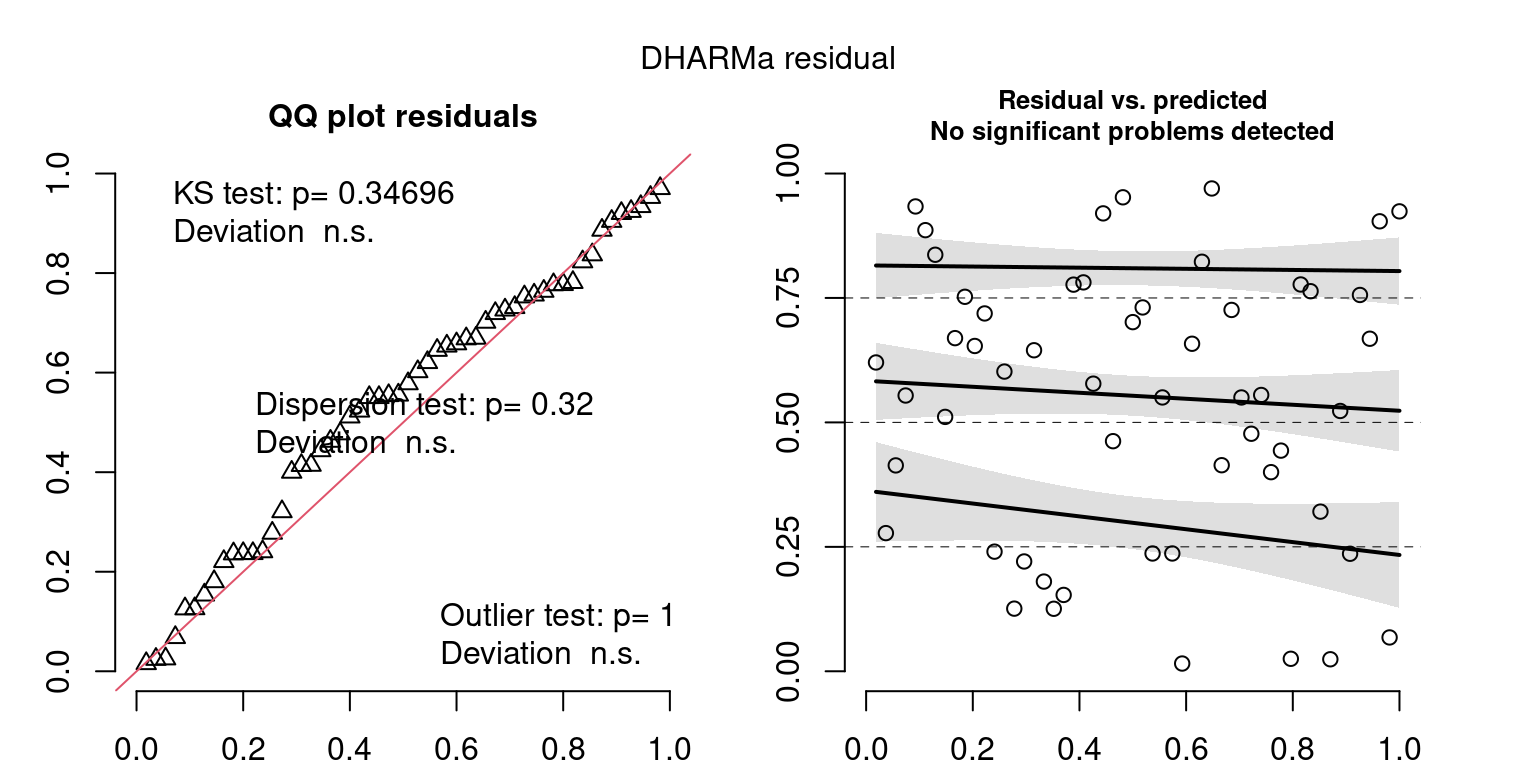
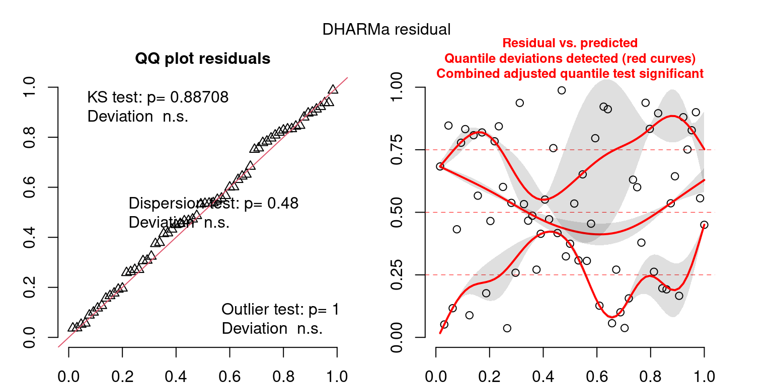
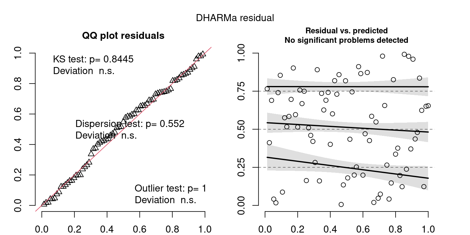
unnest(pred)Checks to ensure models are valid.
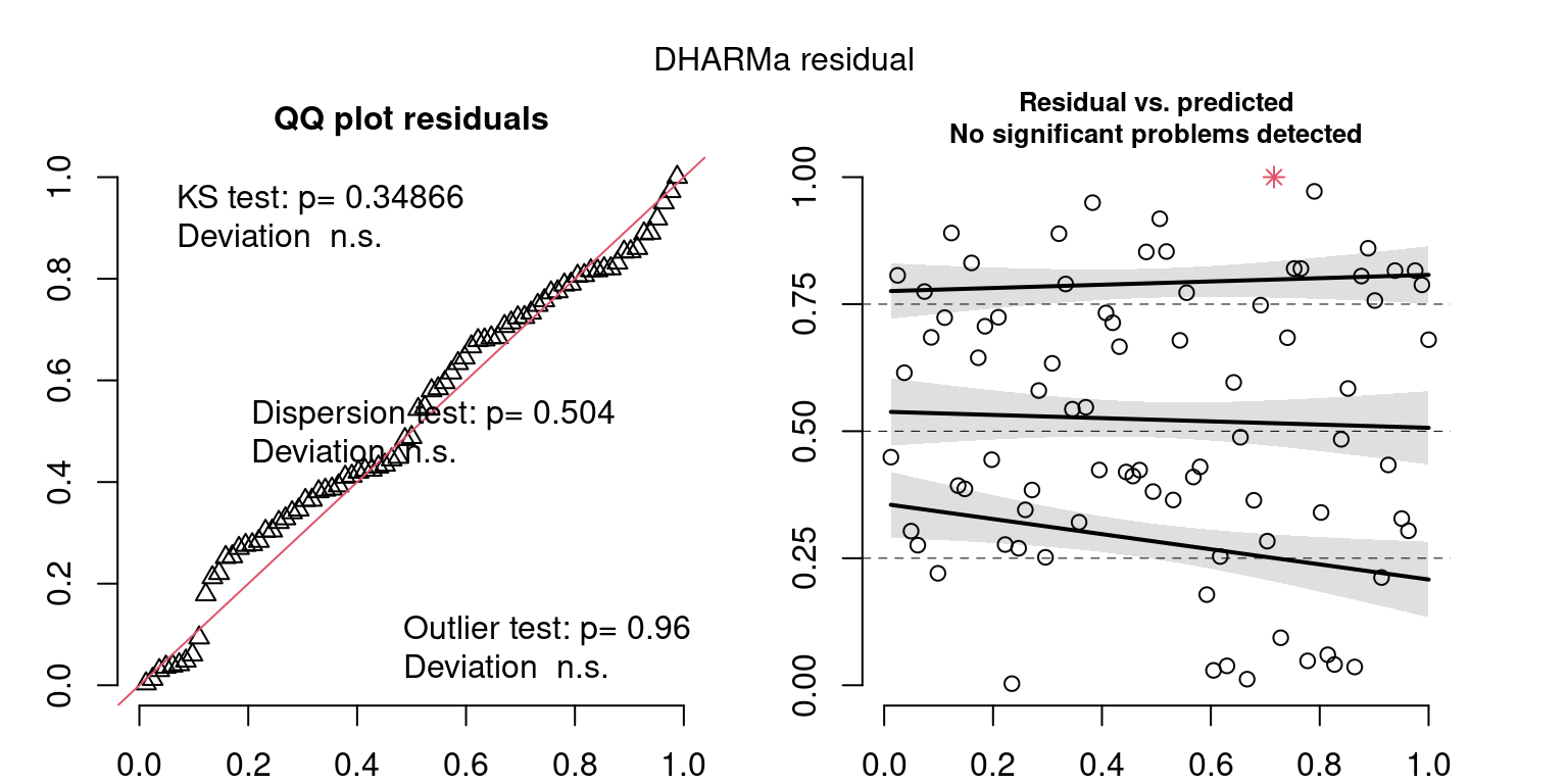
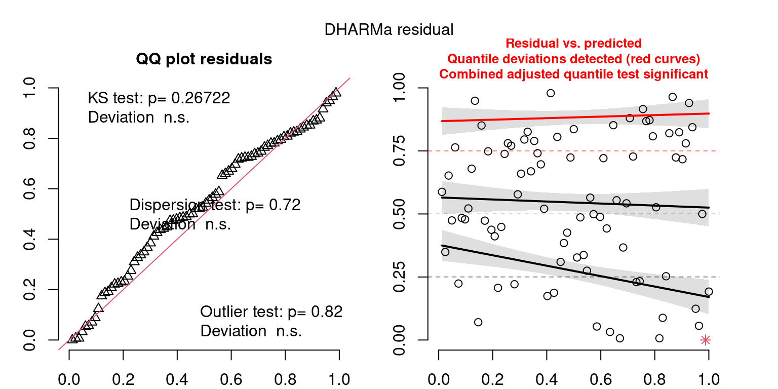
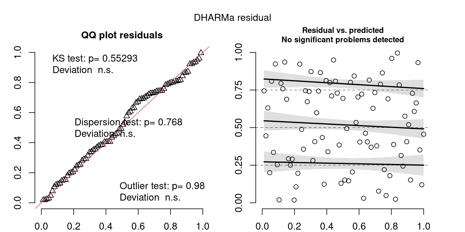
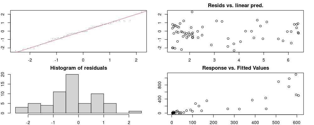
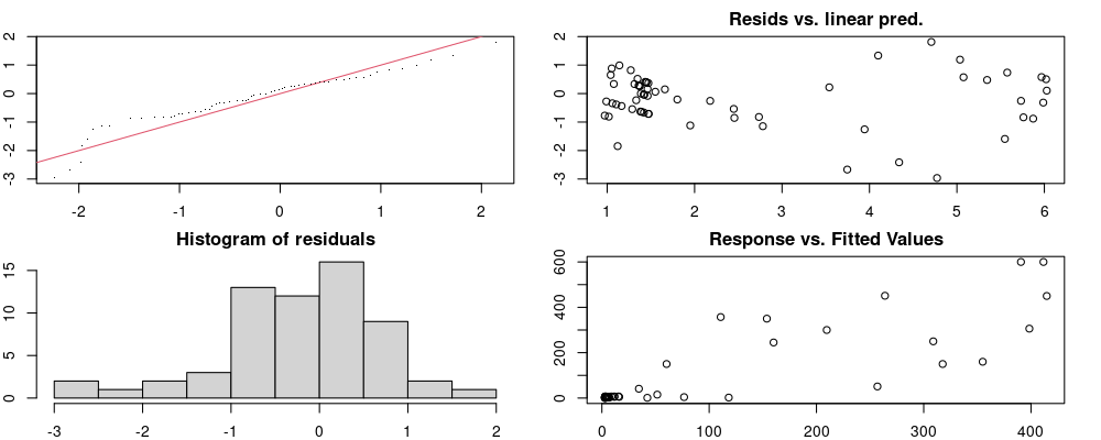
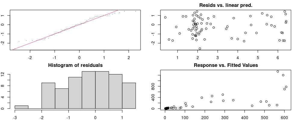
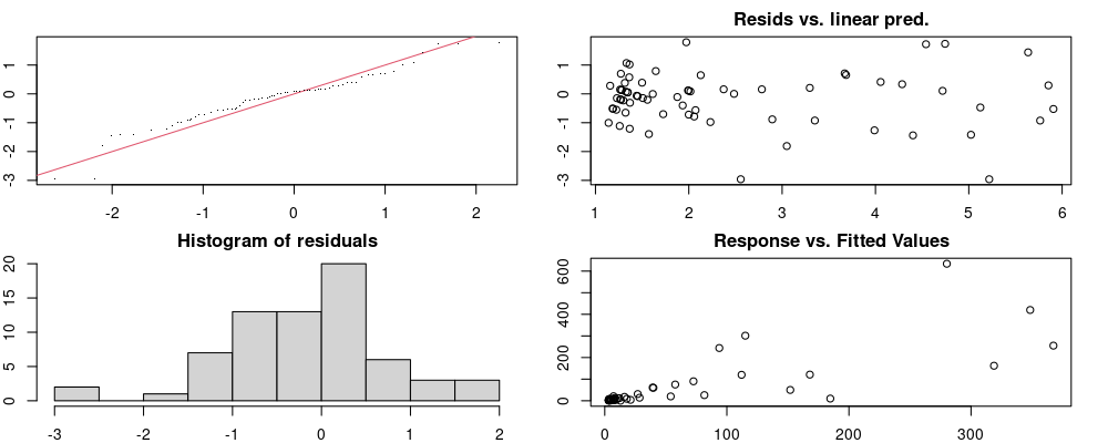
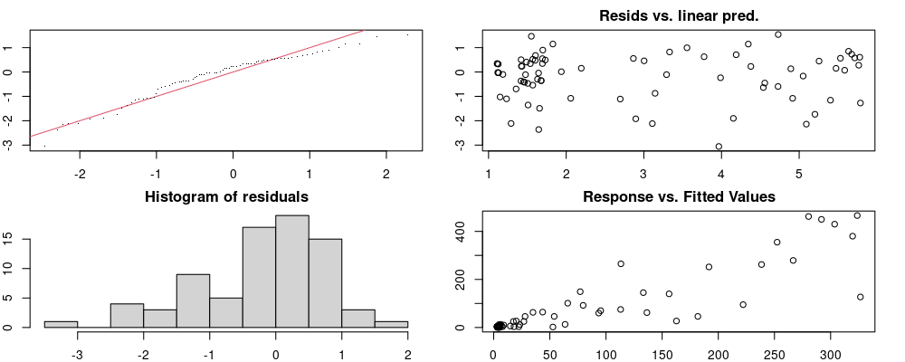
Here we look for two things
- first that there is full convergence
- second that there is not a significant non-random pattern in the residuals around the smoothing term (p-value, but be aware this is an approximation2)
If we have low p-values, we want to check and see
- if the model doesn’t look like it fits the data (see the model plots at the end of this script)
- if the
k(number of basis functions) andedf(effective degrees of freedom) values are similar (if they are, this implies that we haven’t picked a large enoughk)
Code
checks <- gams |>
  mutate(checks = map2(models, year, gam_check)) |>
  invisible() |>
  mutate(plots = map(checks, \(x) pluck(x, "plot")),
         df = map(checks, \(x) pluck(x, "checks"))) |>
  unnest(df) |>
  mutate(low_k = p_value < 0.1)

c <- checks |>
  filter(low_k | !full_convergence) |>
  select(year, param, k, edf, k_index, p_value, convergence)

gt(c)| year | param | k | edf | k_index | p_value | convergence |
|---|---|---|---|---|---|---|
| 2010 | s(doy) | 19.00 | 8.57 | 0.76 | 0.027 | full convergence after 4 iterations. |
| 2012 | s(doy) | 19.00 | 7.68 | 0.76 | 0.021 | full convergence after 4 iterations. |
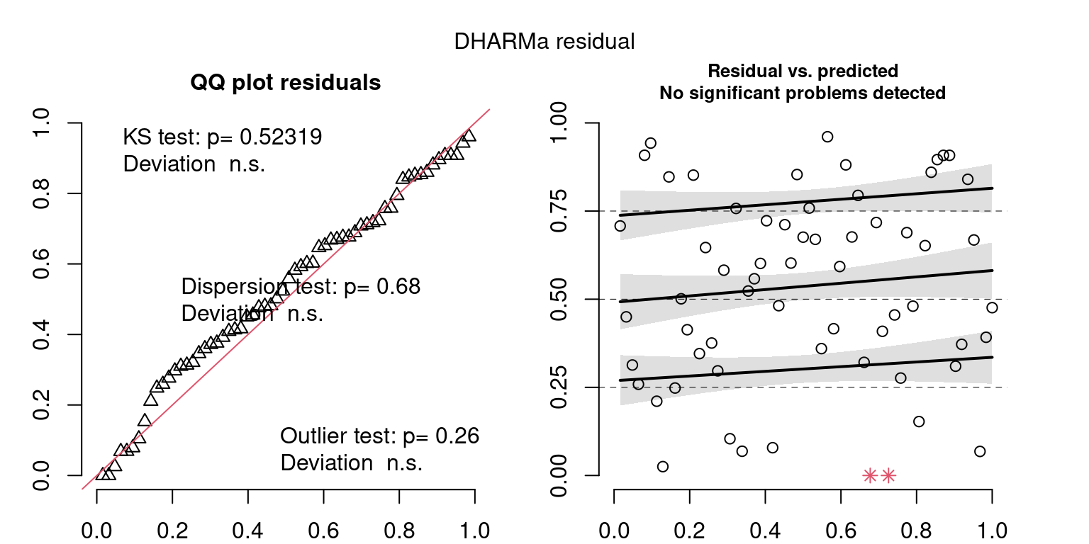
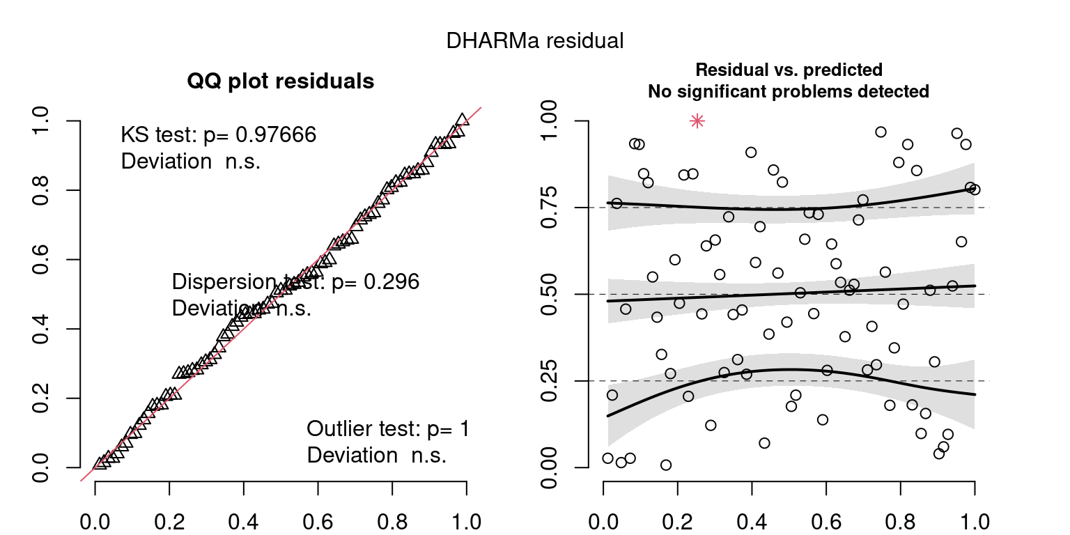
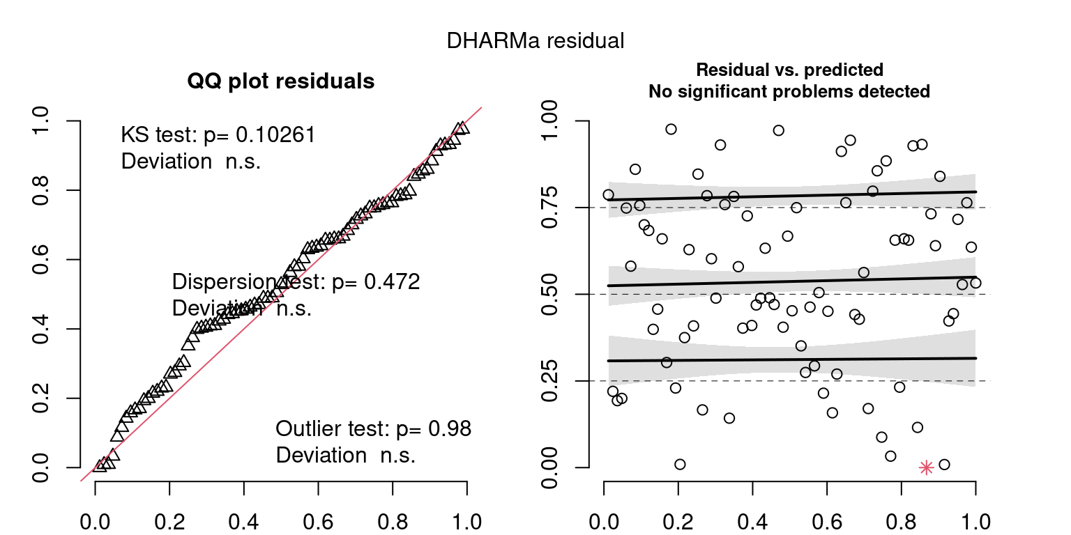
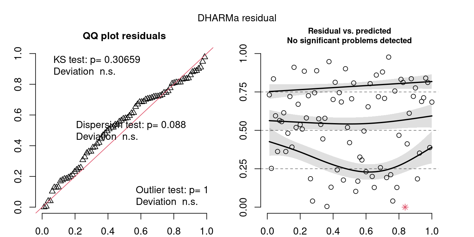
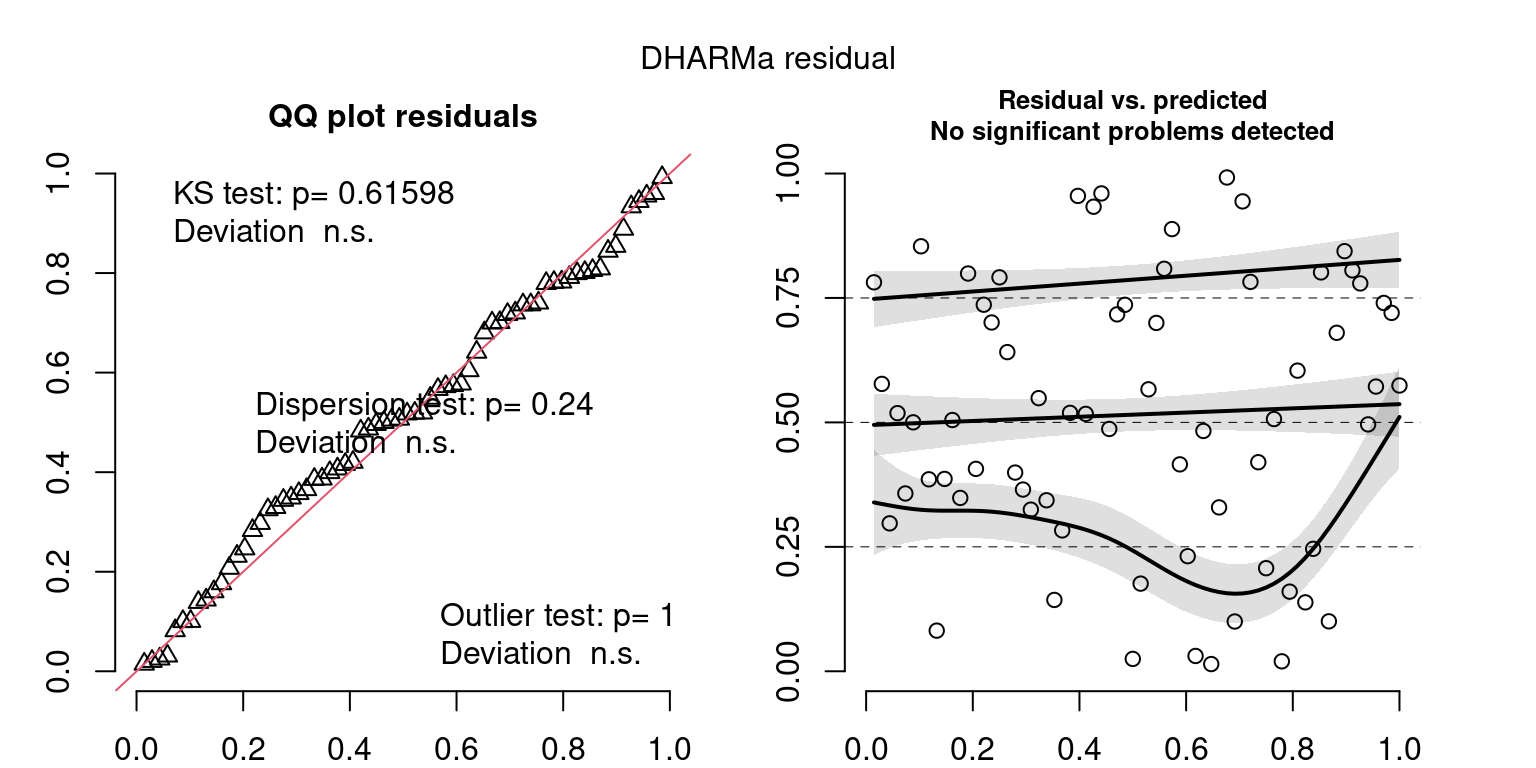
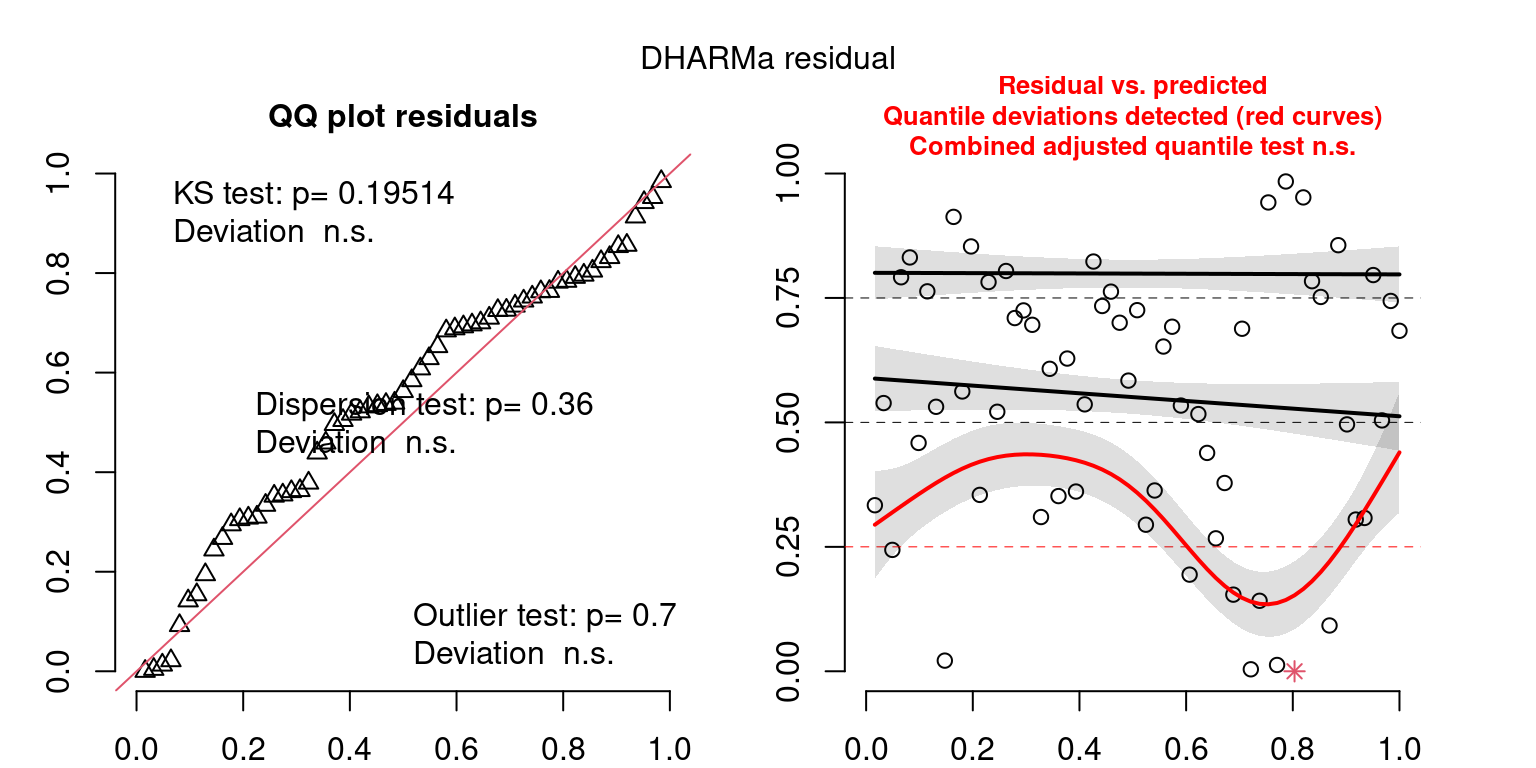
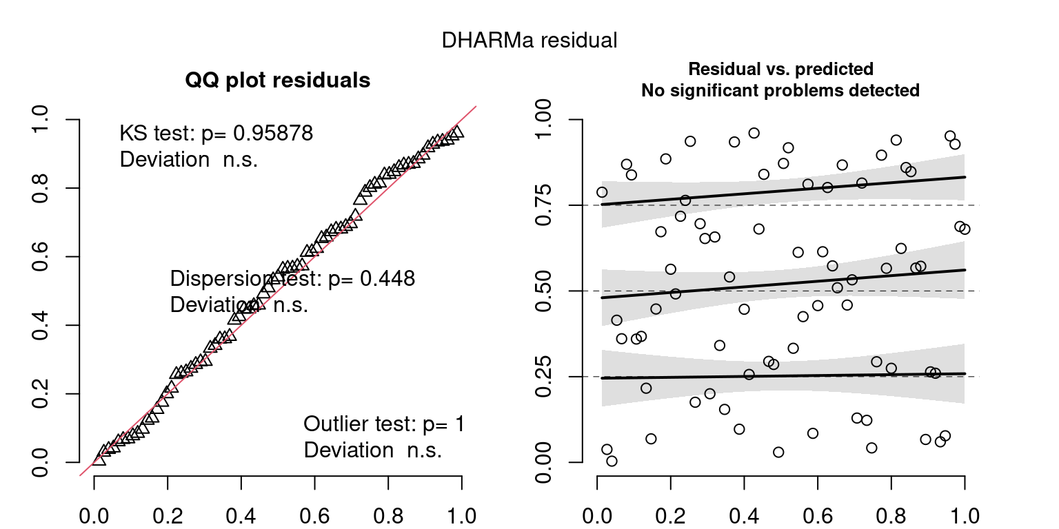
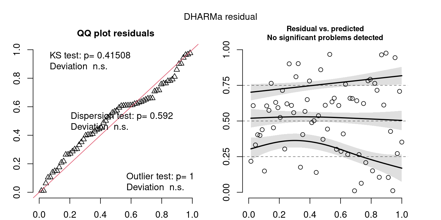
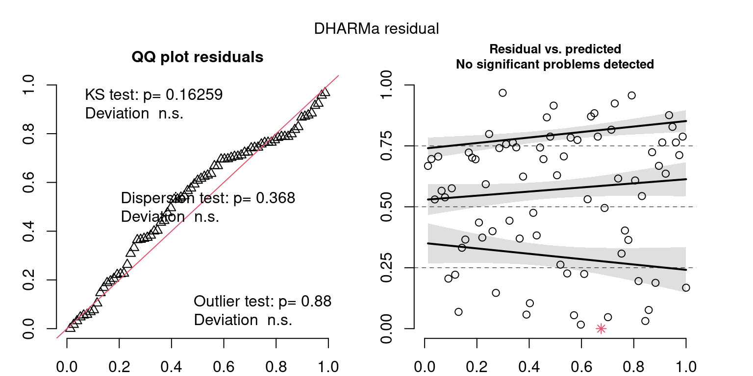
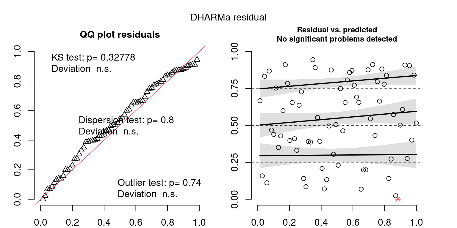
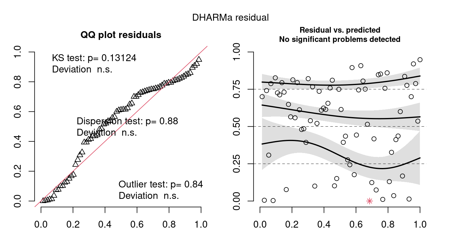
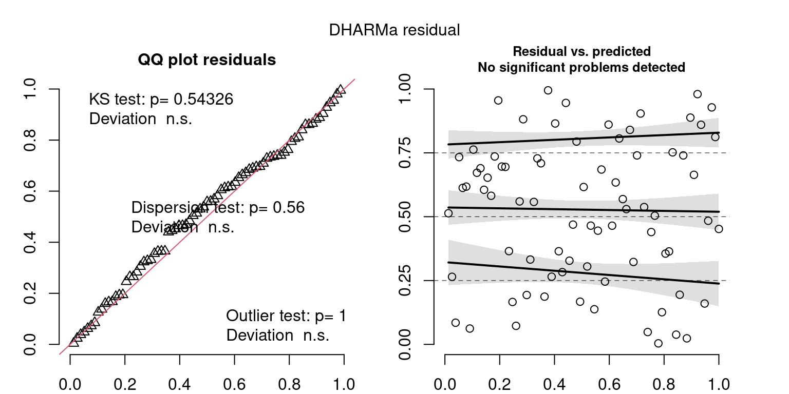
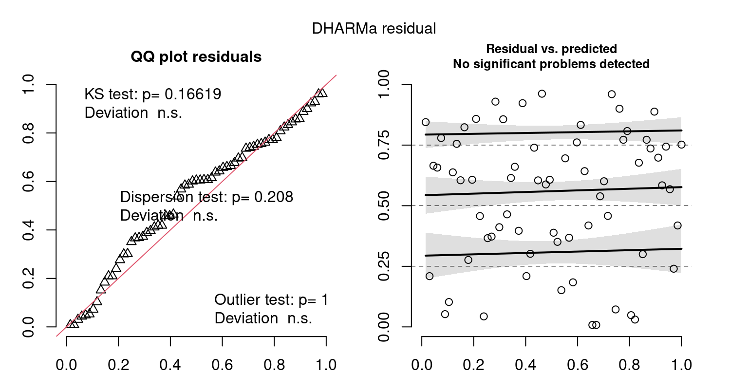
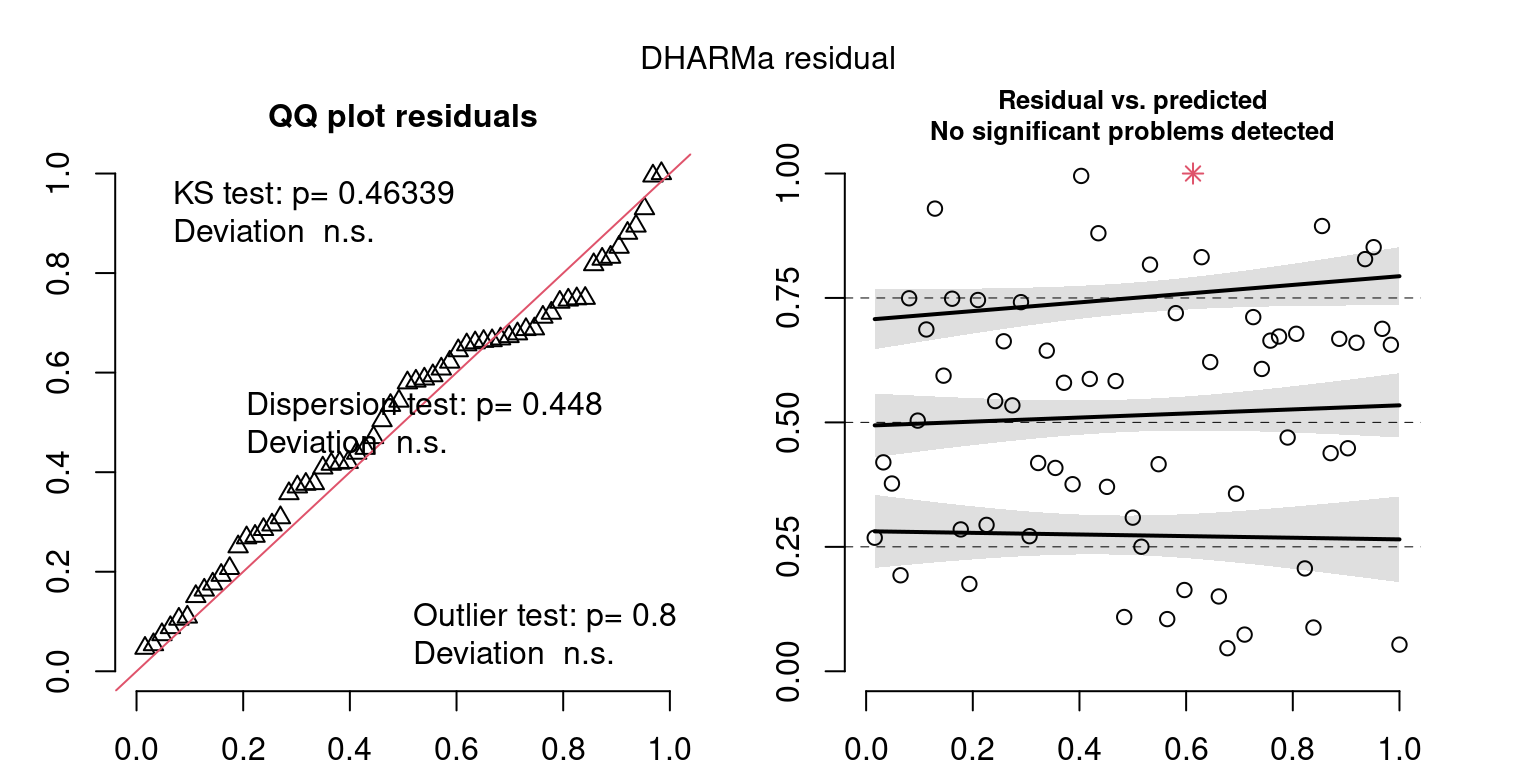
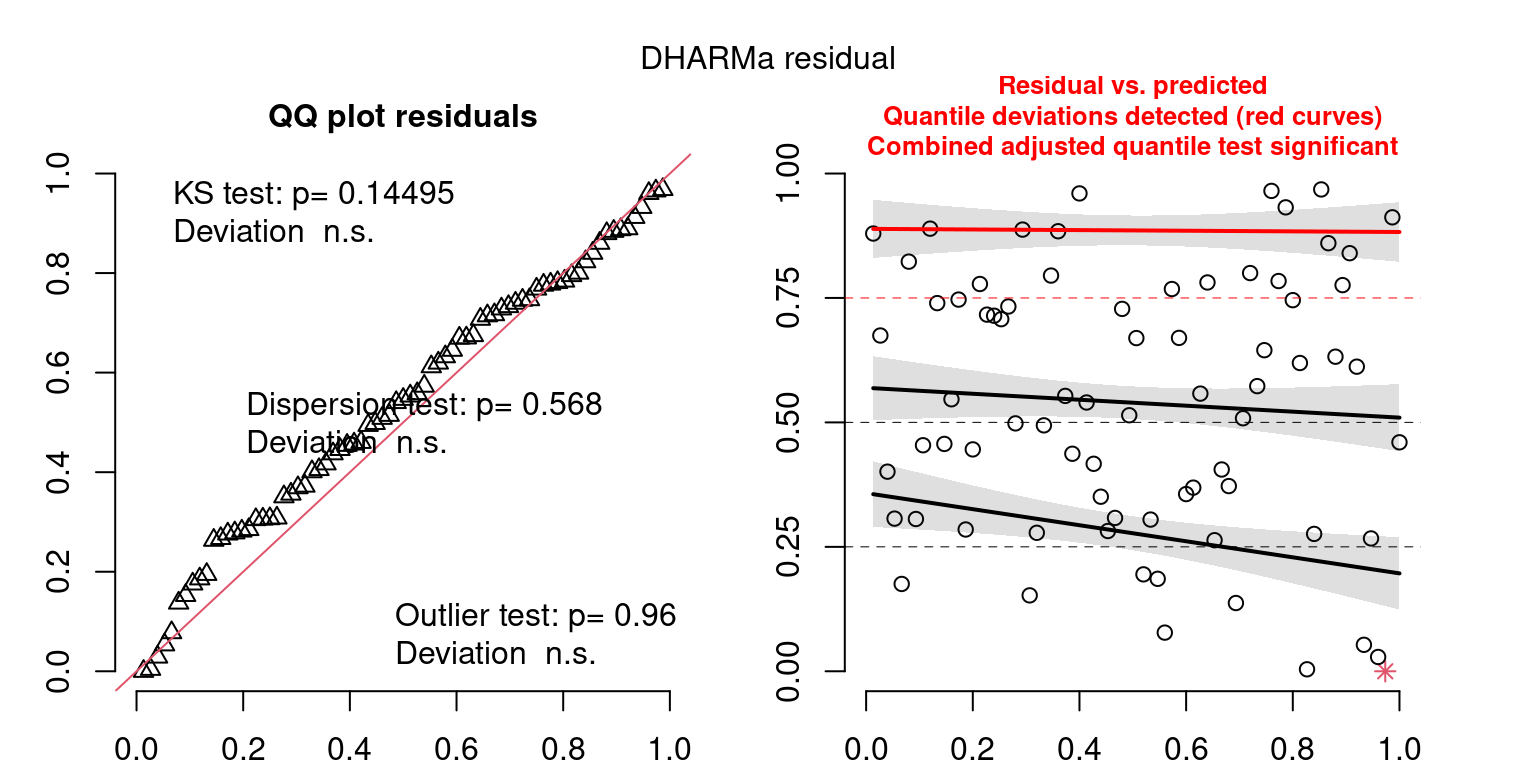
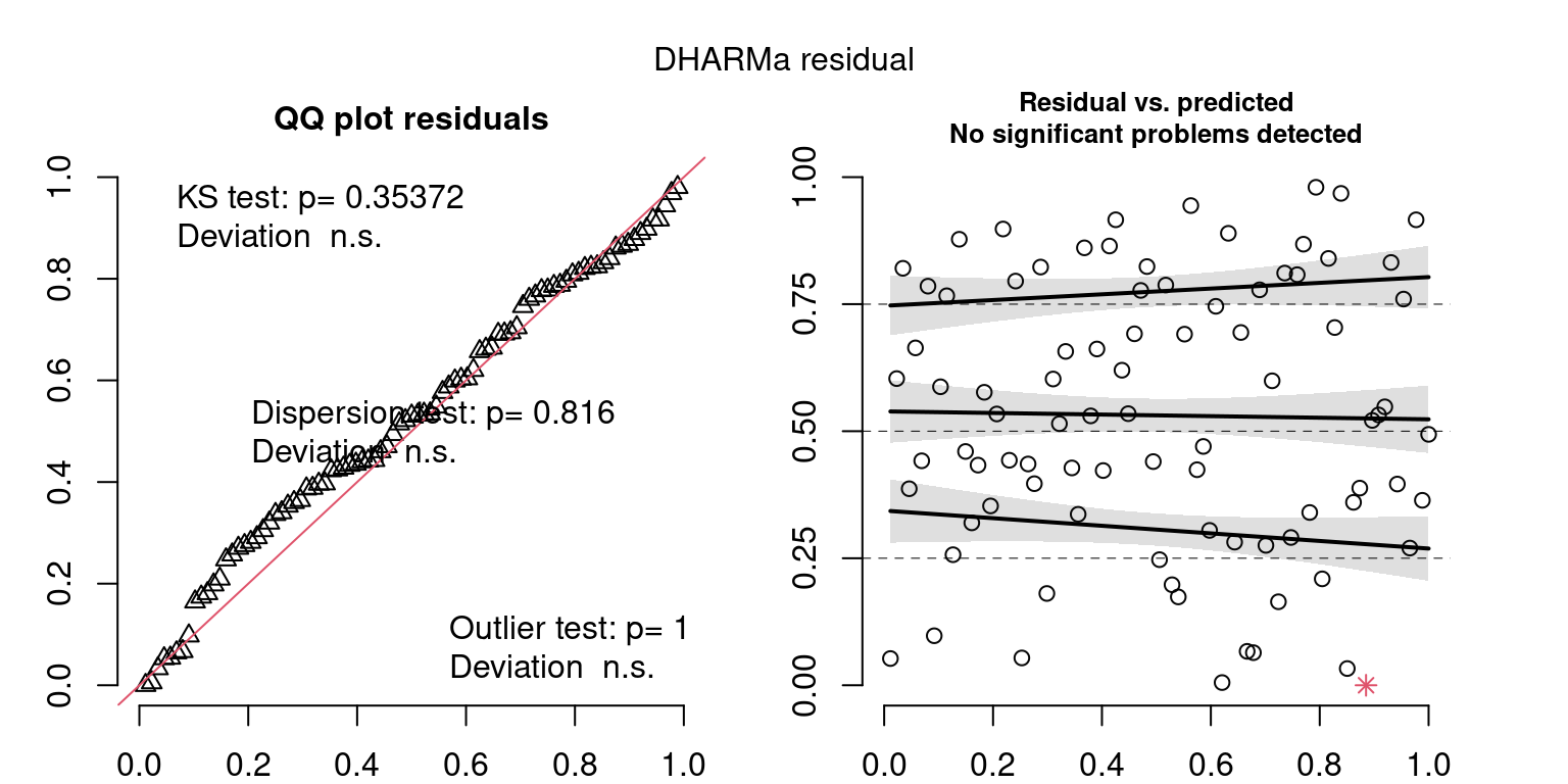
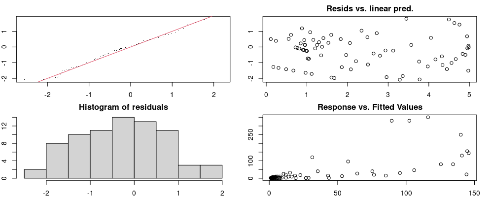
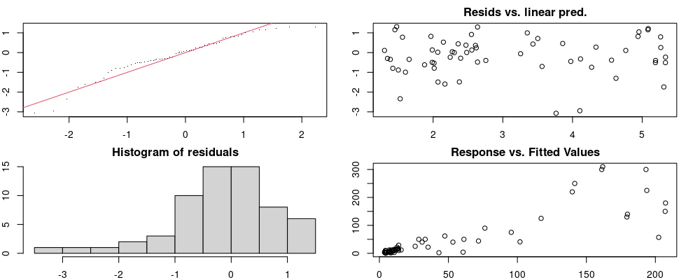
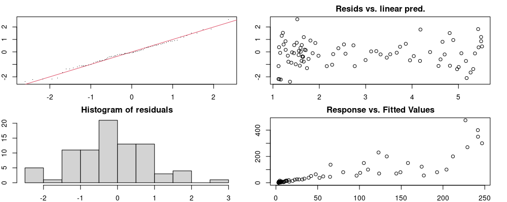
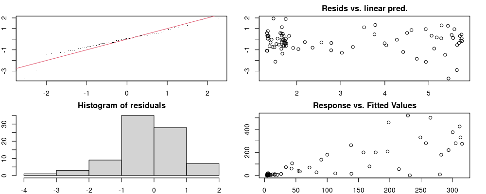
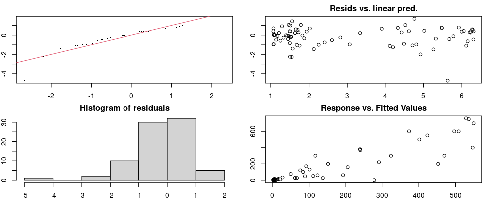
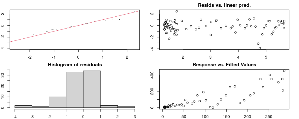
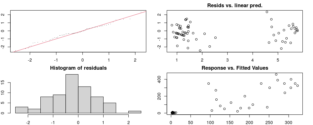
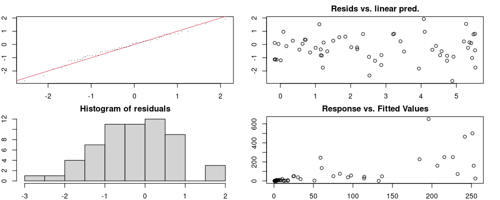
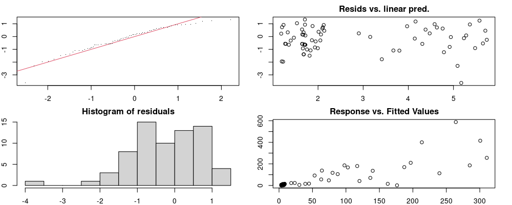
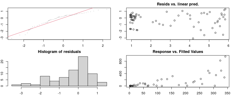
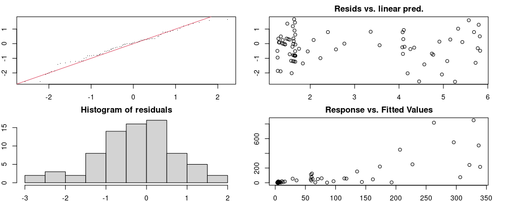
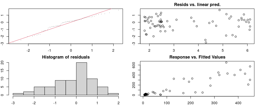
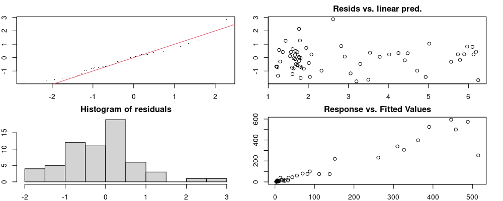
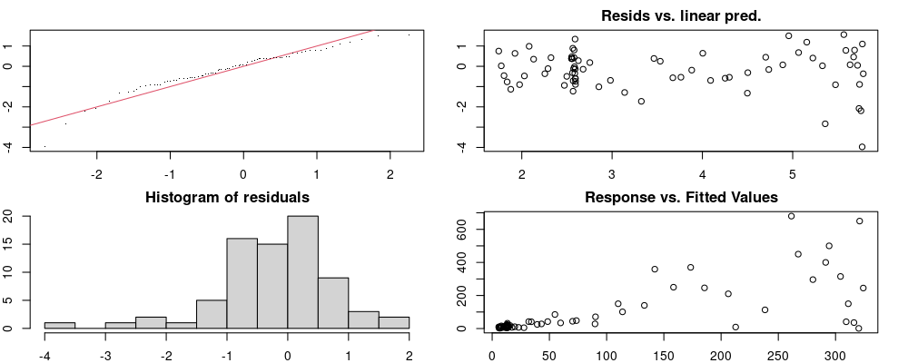
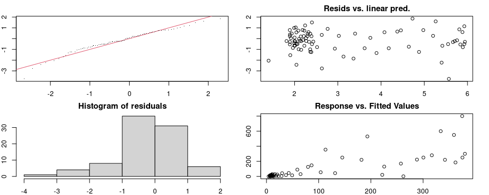
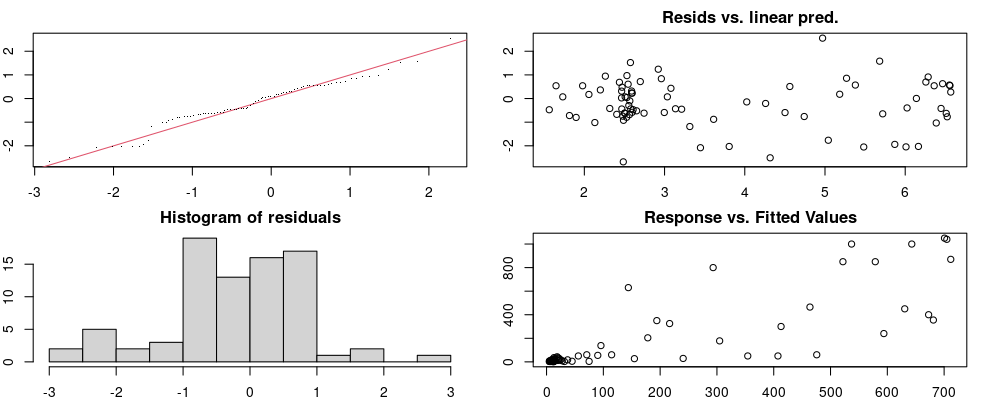
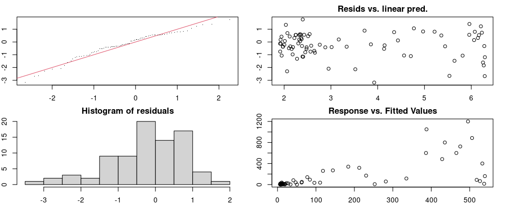
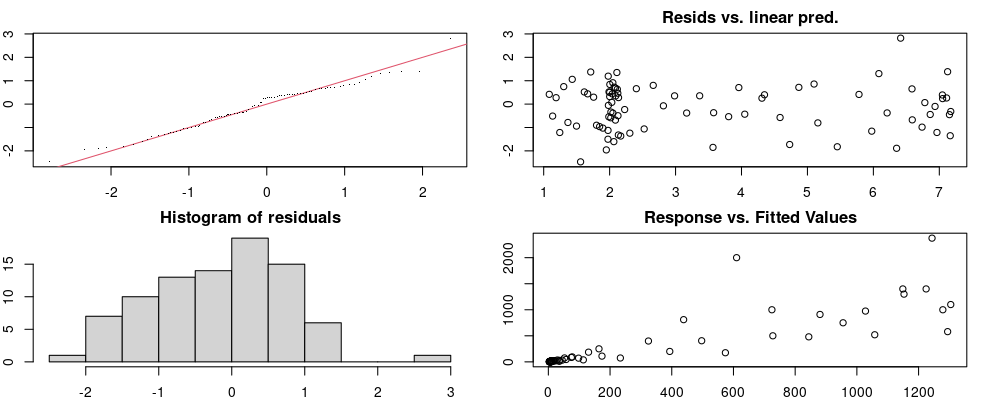
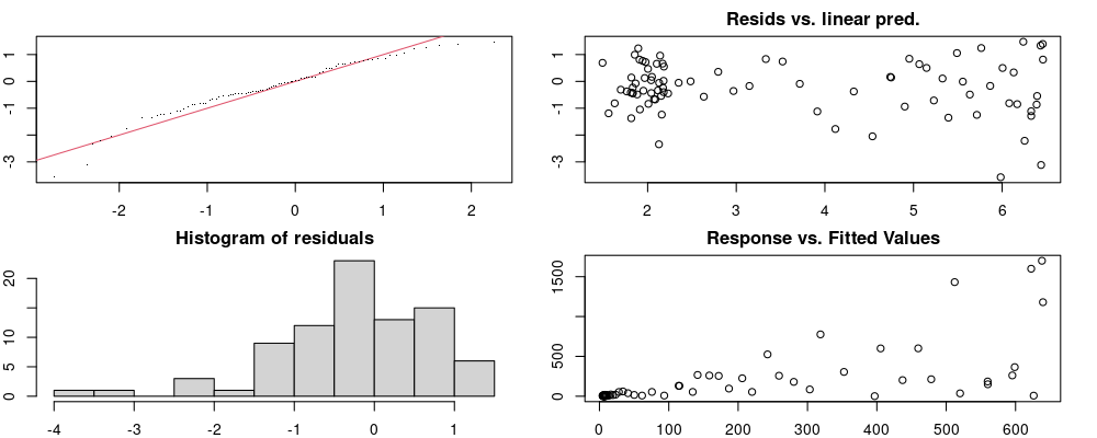
These plots are two different ways of presenting model diagnostics.
gam.check() is the default check that produces both these plots as well as the diagnostics in the Model Evaluation tab.
DHARMa is a package for simulating residuals to allow model checking for all types of models (details).
Both these sets of plots can be interpreted similarly to general linear model plots. We want roughly normal residuals and constant variance.
I tend to put more weight on DHARMa as it’s plots are easier to interpret for non-Gaussian model residuals, but I have included the gam.check() plots for completeness.
Year: 1999
DHARMa’s simulateResiduals() plot
Year: 2000
DHARMa’s simulateResiduals() plot
Year: 2001
DHARMa’s simulateResiduals() plot
Year: 2002
DHARMa’s simulateResiduals() plot
Year: 2003
DHARMa’s simulateResiduals() plot
Year: 2004
DHARMa’s simulateResiduals() plot
Year: 2005
DHARMa’s simulateResiduals() plot
Year: 2006
DHARMa’s simulateResiduals() plot

Year: 2008
DHARMa’s simulateResiduals() plot
Year: 2009
DHARMa’s simulateResiduals() plot

Year: 2010
DHARMa’s simulateResiduals() plot
Year: 2011
DHARMa’s simulateResiduals() plot
Year: 2012
DHARMa’s simulateResiduals() plot
Year: 2013
DHARMa’s simulateResiduals() plot
Year: 2014
DHARMa’s simulateResiduals() plot
Year: 2015
DHARMa’s simulateResiduals() plot
Year: 2016
DHARMa’s simulateResiduals() plot
Year: 2017
DHARMa’s simulateResiduals() plot
Year: 2018
DHARMa’s simulateResiduals() plot
Year: 2019
DHARMa’s simulateResiduals() plot
Year: 2020
DHARMa’s simulateResiduals() plot
Year: 2021
DHARMa’s simulateResiduals() plot
Year: 2022
DHARMa’s simulateResiduals() plot
Year: 2023
DHARMa’s simulateResiduals() plot
Year: 1999
gam.check() plot
Year: 2000
gam.check() plot
Year: 2001
gam.check() plot
Year: 2002
gam.check() plot
Year: 2003
gam.check() plot
Year: 2004
gam.check() plot
Year: 2005
gam.check() plot
Year: 2006
gam.check() plot
Year: 2008
gam.check() plot
Year: 2009
gam.check() plot
Year: 2010
gam.check() plot
Year: 2011
gam.check() plot
Year: 2012
gam.check() plot
Year: 2013
gam.check() plot
Year: 2014
gam.check() plot
Year: 2015
gam.check() plot
Year: 2016
gam.check() plot
Year: 2017
gam.check() plot
Year: 2018
gam.check() plot
Year: 2019
gam.check() plot
Year: 2020
gam.check() plot
Year: 2021
gam.check() plot
Year: 2022
gam.check() plot
Year: 2023
gam.check() plot
Model Validity
Based on the Model Evaluation, there are years with lower k-indices and a p-value < 0.1. It may be worth double checking that these models don’t look too unreasonable.
On the whole, there seems to be quite a bit of variability, but nothing that seems especially problematic.
Code
g <- lapply(c$year, \(y) plot_model(v[v$year == y, ], pred[pred$year == y, ]) +
              labs(title = y))
wrap_plots(g)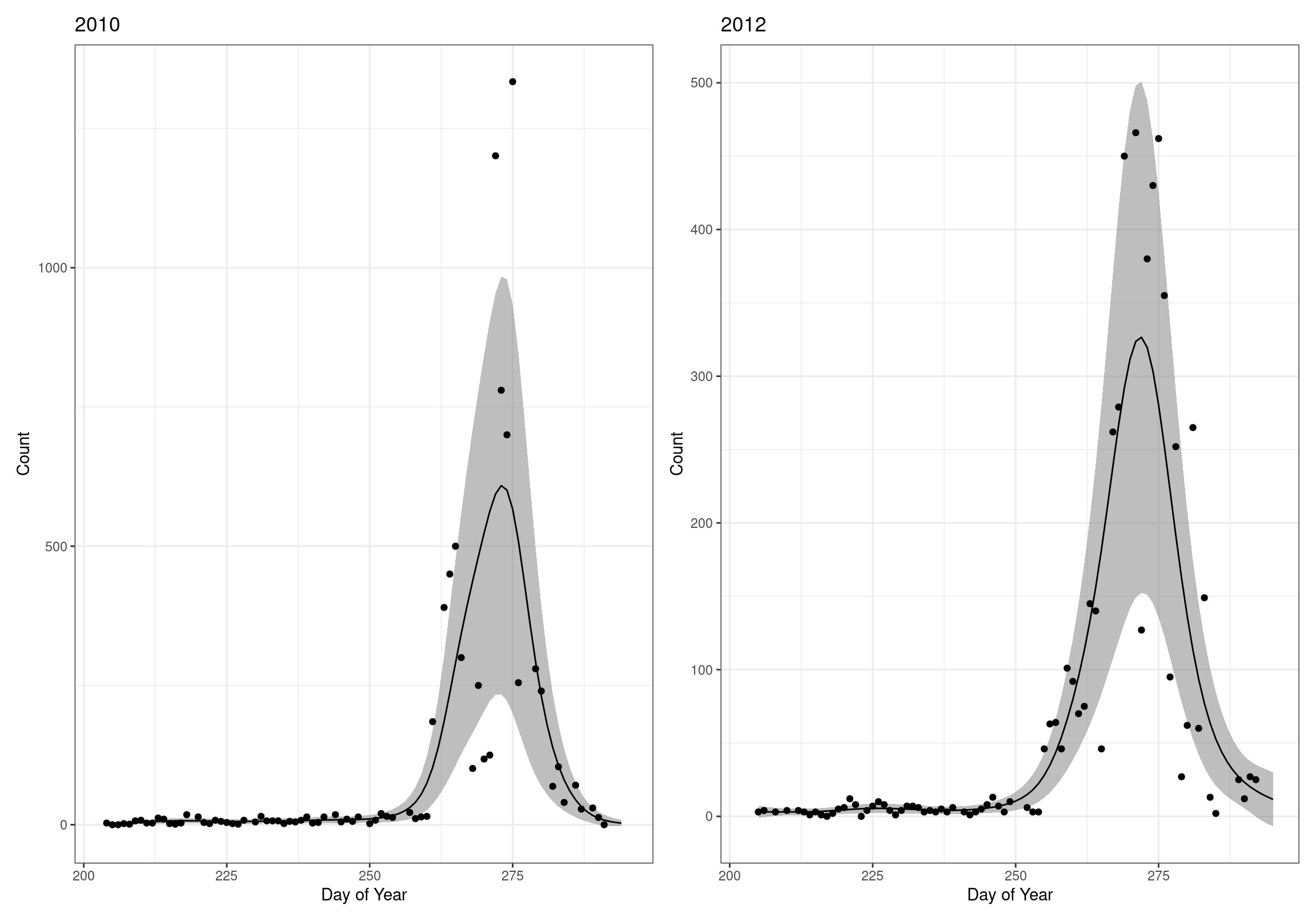
Based on the Model Check Plots, particularly the ones with Simulated DHARMa residuals, we have good model fit (QQ plots of residuals) throughout, but a couple examples of potential non-constant variance. However, I am not very concerned about this for several reasons.
- Although DHARMa highlighted these plots as having significant quantile deviations, visually, I don’t find the deviations that concerning.
- Heteroscedasticity can lead to issues with our Standard Errors, but since we’re only really interested in the predicted value (based on the estimates), these problems don’t really apply to us (we’re not interpreting model error or significance of parameters).
Therefore I suggest we proceed with these models and extract the metrics we’re interested in.
2. Residents
Using a resident date (resident_date) cutoff of DOY 240. Here we calculate the min, max, mean, and median number of residents throughout the ‘resident period’ (from the start to DOY 240).
Note: Resident counts are fractional because they are based on the predicted counts from the GAM models (i.e. the smoothed curve).
residents <- pred |>
  filter(doy < resident_date) |>
  group_by(year) |>
  # Calculate resident statistics by year
  summarize(res_pop_min = min(count),
            res_pop_max = max(count),
            res_pop_median = median(count),
            res_pop_mean = mean(count)) |>
  # Round to 1 decimal place
mutate(across(starts_with("res"), \(x) round(x, 1)))gt(residents)| year | res_pop_min | res_pop_max | res_pop_median | res_pop_mean |
|---|---|---|---|---|
| 1999 | 3.7 | 8.4 | 4.6 | 5.5 |
| 2000 | 1.1 | 4.6 | 2.5 | 2.5 |
| 2001 | 3.7 | 14.1 | 7.4 | 8.1 |
| 2002 | 3.1 | 5.7 | 4.4 | 4.3 |
| 2003 | 3.8 | 5.8 | 4.7 | 4.7 |
| 2004 | 2.9 | 5.1 | 4.3 | 4.0 |
| 2005 | 3.8 | 5.9 | 4.3 | 4.6 |
| 2006 | 2.2 | 4.4 | 3.2 | 3.3 |
| 2008 | 0.9 | 3.4 | 1.5 | 1.8 |
| 2009 | 2.6 | 4.4 | 3.4 | 3.4 |
| 2010 | 1.5 | 7.6 | 6.3 | 5.7 |
| 2011 | 3.2 | 5.3 | 3.7 | 3.8 |
| 2012 | 3.0 | 5.5 | 4.2 | 4.2 |
| 2013 | 3.4 | 8.5 | 5.5 | 6.0 |
| 2014 | 2.5 | 3.6 | 2.7 | 2.9 |
| 2015 | 3.5 | 5.3 | 4.7 | 4.6 |
| 2016 | 6.1 | 11.8 | 9.4 | 9.2 |
| 2017 | 3.3 | 8.0 | 5.2 | 5.1 |
| 2018 | 5.7 | 13.4 | 11.3 | 10.6 |
| 2019 | 6.6 | 11.1 | 8.0 | 8.4 |
| 2020 | 4.8 | 13.4 | 11.8 | 10.8 |
| 2021 | 6.8 | 13.2 | 9.1 | 9.3 |
| 2022 | 3.0 | 8.5 | 7.2 | 6.4 |
| 2023 | 4.4 | 8.9 | 7.1 | 7.2 |
3. Cumulative counts
Here we calculate cumulative counts after subtracting the median resident population.
As noted in our initial exploration, if we calculate cumulative accounts across the whole year, we include cumulative counts of residents which could bias the start of migration to an earlier date.
Therefore, we subtract the median number of resident birds from each daily count and then calculate the cumulative number of birds seen in kettles and use this cumulative curve to calculate our metrics of migration (calculated in the following sections).
Because we are subtracting a median value from the whole data range within a year we can occasionally get some funny counts (i.e. if the number of resident vultures fluctuated between 2 and 4, this would mean that subtracting a median of 3 would sometimes result in a negative count which in turn would mean that the cumulative count would sometimes go down, rather than up).
However, after reviewing the cumulative count figures for all years, I’ve added one more rule: we only start cumulative counts after DOY of 240. This is still very much before the start of migration, but avoids cumulative counts during the very clearly resident period. It helps avoid some of the more extreme negative cumulative counts. Doing this doesn’t appreciably alter the metrics calculated, but seems more reasonable. So gives me more peace of mind.
Overall: I’m not concerned about minor negative cumulative count blips because a) they are minor, and b) they only occur during the resident phase. As soon as the birds start accumulating for migration, the number of birds present is above the resident number fluctuations and the cumulative count accumulates.
Also Note: Counts are fractional because they are based on the predicted counts from the GAM models (i.e. the smoothed curve).
cum_counts <- pred |>
  left_join(select(residents, year, res_pop_median), by = "year") |>
  group_by(year) |>
  mutate(count_init = count,
         count = count - res_pop_median, # Subtract residents from predicted counts
         count = if_else(doy < resident_date, 0, count),
         count_sum = cumsum(count)) |> # Calculate cumulative sum
  ungroup() |>
  select(year, doy, res_pop_median, count_init, count, count_sum)
Showing only a snapshot of the middle of the year 1999.
count_initis the predicted daily kettle count (only included here for illustration)countis the predicted daily kettle count after residents are removed (this means that negative counts are possible before migration starts).count_sumis the cumulative sum of thecountcolumn (this means that it can decrease if counts are negative before migration starts).
Note: the first couple of counts are zero because they take place before the resident date cutoff (240), and have been set to zero so we start cumulative counts on 240.
The median number of residents for 1999 is 4.6
gt(slice(cum_counts, 35:60))| year | doy | res_pop_median | count_init | count | count_sum |
|---|---|---|---|---|---|
| 1999 | 238 | 4.6 | 4.457062 | 0.0000000 | 0.0000000 |
| 1999 | 239 | 4.6 | 4.624695 | 0.0000000 | 0.0000000 |
| 1999 | 240 | 4.6 | 4.818115 | 0.2181154 | 0.2181154 |
| 1999 | 241 | 4.6 | 5.035076 | 0.4350758 | 0.6531912 |
| 1999 | 242 | 4.6 | 5.272257 | 0.6722571 | 1.3254484 |
| 1999 | 243 | 4.6 | 5.527974 | 0.9279740 | 2.2534224 |
| 1999 | 244 | 4.6 | 5.812629 | 1.2126292 | 3.4660516 |
| 1999 | 245 | 4.6 | 6.153038 | 1.5530377 | 5.0190893 |
| 1999 | 246 | 4.6 | 6.590825 | 1.9908247 | 7.0099139 |
| 1999 | 247 | 4.6 | 7.177578 | 2.5775779 | 9.5874918 |
| 1999 | 248 | 4.6 | 7.968728 | 3.3687283 | 12.9562201 |
| 1999 | 249 | 4.6 | 9.021757 | 4.4217568 | 17.3779769 |
| 1999 | 250 | 4.6 | 10.412951 | 5.8129509 | 23.1909278 |
| 1999 | 251 | 4.6 | 12.246878 | 7.6468781 | 30.8378059 |
| 1999 | 252 | 4.6 | 14.656202 | 10.0562023 | 40.8940082 |
| 1999 | 253 | 4.6 | 17.815874 | 13.2158736 | 54.1098818 |
| 1999 | 254 | 4.6 | 21.964218 | 17.3642181 | 71.4740999 |
| 1999 | 255 | 4.6 | 27.448787 | 22.8487866 | 94.3228865 |
| 1999 | 256 | 4.6 | 34.779072 | 30.1790719 | 124.5019584 |
| 1999 | 257 | 4.6 | 44.671167 | 40.0711665 | 164.5731249 |
| 1999 | 258 | 4.6 | 58.061065 | 53.4610653 | 218.0341902 |
| 1999 | 259 | 4.6 | 76.051163 | 71.4511634 | 289.4853536 |
| 1999 | 260 | 4.6 | 99.777668 | 95.1776678 | 384.6630214 |
| 1999 | 261 | 4.6 | 130.271456 | 125.6714561 | 510.3344775 |
| 1999 | 262 | 4.6 | 168.225334 | 163.6253336 | 673.9598111 |
| 1999 | 263 | 4.6 | 213.860507 | 209.2605071 | 883.2203182 |
These figures show the early part of the migration season with predicted daily counts (red) overlaid with the adjusted cumulative predicted counts (grey).
- Red bars are predicted non-cumulative initial counts (no subtractions made)
- Grey bars are cumulative predicted counts created after subtracting resident birds from each daily count. Accumulating only after 240.
- Note that there is a little negative cumulative blip in 2013 that evens out relatively quickly.
ggplot(data = filter(cum_counts, doy < 265), aes(x = doy, y = count_sum)) +
  theme_bw() +
  geom_bar(aes(y = count_init), stat = "identity", fill = "red", alpha = 0.8) +
  geom_bar(stat = "identity", alpha = 0.5) +
  #geom_bar(aes(y = count), stat = "identity", fill = "blue", alpha = 0.5) +
  facet_wrap(~ year, scales = "free_y")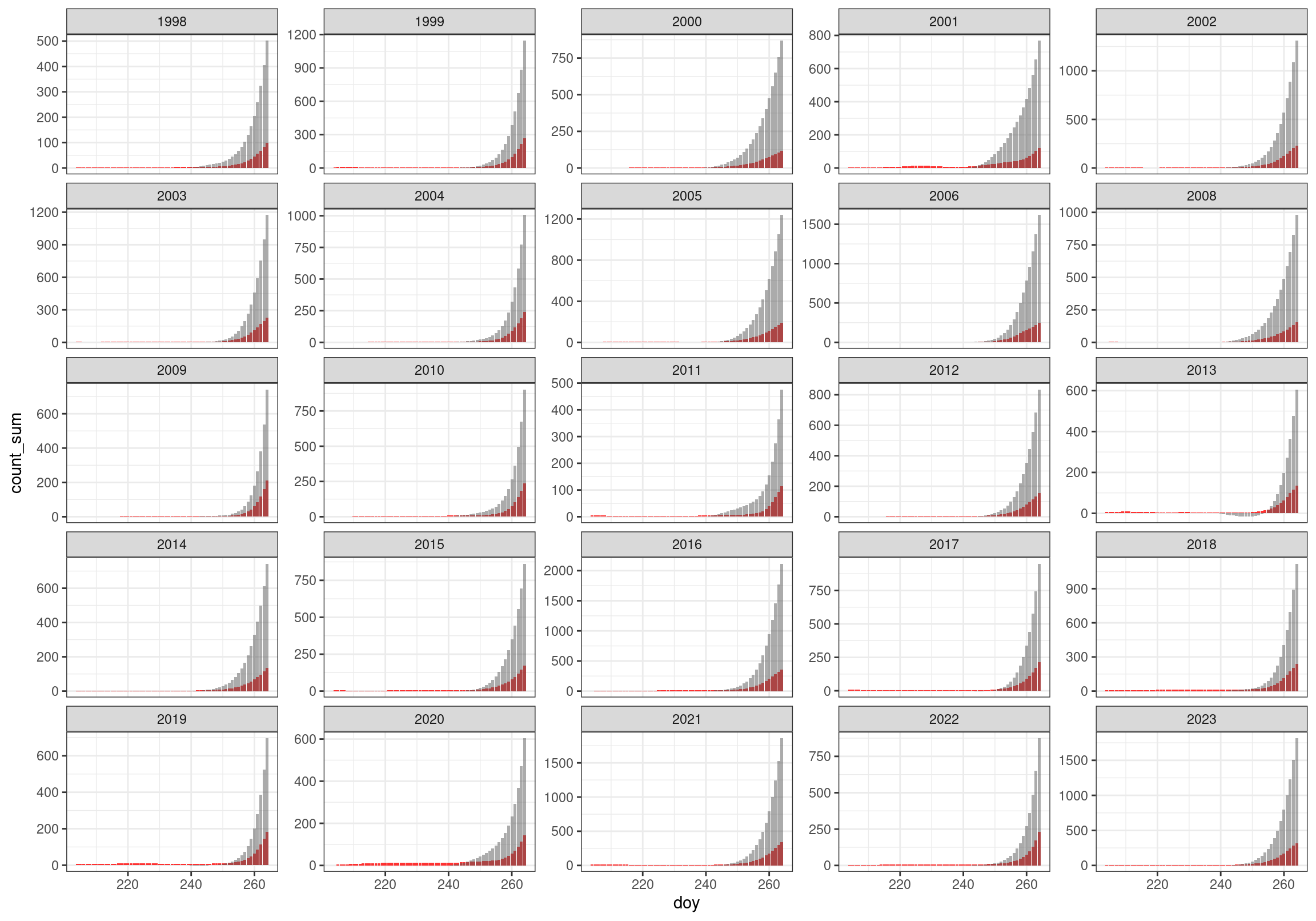
4. Dates of passage
Now that we have the cumulative predicted counts, we can calculate the dates at which a particular proportion of the migrating population had passed through.
Here we look at the dates at which 5%, 25%, 50%, 75%, and 95% of the birds have passed through.
We also calculate the date at which the predicted count was at it’s maximum.
The 5-95% and 25-75% date rages will then be used to calculate duration of passage, population sizes, and migration patterns in the next sections.
max_passage <- pred |>
  group_by(year) |>
  # Keep first max count
  slice_max(count, with_ties = FALSE) |>
  mutate(measure = "max") |>
  select(year, measure, doy_passage = doy)

dts <- cum_counts |>
  select(year, doy, count, count_sum) |>
  group_by(year) |>
  calc_dates() |>
  rename("measure" = "perc") |>
  bind_rows(max_passage) |>
  arrange(year, measure)
Only showing part of the data.
gt(slice(dts, 1:30))| year | measure | count_thresh | doy_passage | count_pred |
|---|---|---|---|---|
| 1999 | max | NA | 271 | NA |
| 1999 | p05 | 431.3002 | 261 | 125.67146 |
| 1999 | p25 | 2156.5009 | 267 | 448.50778 |
| 1999 | p50 | 4313.0019 | 271 | 603.35750 |
| 1999 | p75 | 6469.5028 | 275 | 446.10741 |
| 1999 | p95 | 8194.7035 | 282 | 109.70742 |
| 2000 | max | NA | 269 | NA |
| 2000 | p05 | 136.1183 | 253 | 25.80135 |
| 2000 | p25 | 680.5916 | 262 | 95.98933 |
| 2000 | p50 | 1361.1831 | 268 | 138.06548 |
| 2000 | p75 | 2041.7747 | 273 | 116.72027 |
| 2000 | p95 | 2586.2479 | 281 | 32.13846 |
| 2001 | max | NA | 271 | NA |
| 2001 | p05 | 161.7092 | 254 | 27.60036 |
| 2001 | p25 | 808.5459 | 265 | 126.37183 |
| 2001 | p50 | 1617.0917 | 270 | 197.69425 |
| 2001 | p75 | 2425.6376 | 274 | 172.39983 |
| 2001 | p95 | 3072.4743 | 280 | 52.30889 |
| 2002 | max | NA | 266 | NA |
| 2002 | p05 | 223.0923 | 257 | 60.39372 |
| 2002 | p25 | 1115.4614 | 264 | 222.46137 |
| 2002 | p50 | 2230.9229 | 268 | 224.84705 |
| 2002 | p75 | 3346.3843 | 275 | 119.12477 |
| 2002 | p95 | 4238.7535 | 285 | 60.99240 |
| 2003 | max | NA | 269 | NA |
| 2003 | p05 | 295.8550 | 259 | 85.83200 |
| 2003 | p25 | 1479.2748 | 266 | 277.49744 |
| 2003 | p50 | 2958.5497 | 271 | 300.54305 |
| 2003 | p75 | 4437.8245 | 276 | 227.34231 |
| 2003 | p95 | 5621.2443 | 284 | 78.15856 |
5. Duration of passage
Duration of passage is calculated as the number of days between the 5% and 95% (migration) and the 25% and 75% (peak migration) dates.
We also organize the dates of passage into separate columns in this step.
passage <- dts |>
  group_by(year) |>
  summarize(mig_start_doy = doy_passage[measure == "p05"],
            mig_end_doy = doy_passage[measure == "p95"],
            peak_start_doy = doy_passage[measure == "p25"],
            peak_end_doy = doy_passage[measure == "p75"],
            p50_doy = doy_passage[measure == "p50"],
            max_doy = doy_passage[measure == "max"],
            mig_dur_days = mig_end_doy - mig_start_doy,
peak_dur_days = peak_end_doy - peak_start_doy)gt(passage)| year | mig_start_doy | mig_end_doy | peak_start_doy | peak_end_doy | p50_doy | max_doy | mig_dur_days | peak_dur_days |
|---|---|---|---|---|---|---|---|---|
| 1999 | 261 | 282 | 267 | 275 | 271 | 271 | 21 | 8 |
| 2000 | 253 | 281 | 262 | 273 | 268 | 269 | 28 | 11 |
| 2001 | 254 | 280 | 265 | 274 | 270 | 271 | 26 | 9 |
| 2002 | 257 | 285 | 264 | 275 | 268 | 266 | 28 | 11 |
| 2003 | 259 | 284 | 266 | 276 | 271 | 269 | 25 | 10 |
| 2004 | 262 | 288 | 268 | 278 | 273 | 272 | 26 | 10 |
| 2005 | 256 | 283 | 265 | 275 | 270 | 270 | 27 | 10 |
| 2006 | 257 | 282 | 264 | 275 | 270 | 270 | 25 | 11 |
| 2008 | 256 | 281 | 265 | 275 | 270 | 271 | 25 | 10 |
| 2009 | 261 | 277 | 266 | 272 | 269 | 269 | 16 | 6 |
| 2010 | 262 | 282 | 268 | 276 | 272 | 273 | 20 | 8 |
| 2011 | 263 | 286 | 270 | 280 | 276 | 277 | 23 | 10 |
| 2012 | 259 | 284 | 267 | 276 | 272 | 272 | 25 | 9 |
| 2013 | 262 | 287 | 269 | 280 | 274 | 275 | 25 | 11 |
| 2014 | 260 | 288 | 269 | 280 | 274 | 274 | 28 | 11 |
| 2015 | 259 | 289 | 267 | 276 | 271 | 270 | 30 | 9 |
| 2016 | 258 | 285 | 265 | 276 | 270 | 271 | 27 | 11 |
| 2017 | 261 | 280 | 267 | 275 | 271 | 272 | 19 | 8 |
| 2018 | 260 | 285 | 267 | 278 | 272 | 270 | 25 | 11 |
| 2019 | 262 | 282 | 267 | 276 | 271 | 271 | 20 | 9 |
| 2020 | 264 | 288 | 272 | 281 | 277 | 277 | 24 | 9 |
| 2021 | 258 | 281 | 266 | 275 | 271 | 271 | 23 | 9 |
| 2022 | 265 | 285 | 271 | 279 | 275 | 276 | 20 | 8 |
| 2023 | 259 | 286 | 268 | 278 | 273 | 274 | 27 | 10 |
6. Population size
Here we calculate population size metrics for different stages of the migration
- Residents (before resident date cutoff [DOY 240])
- Migrants (between migration start [5%] and migration end [95%])
- Ambiguous (between resident date cutoff and migration start as well as after migration end)
- Peak migrants (between peak start [25%] and peak end [75%])
- Raw counts for migrants and peak migrants (min, mean, median, max, total)
- These are the counts recorded by observers in the field
- Remember that total is affected by missing dates
Note: I don’t expect to use the ambiguous category, but have included it for completeness and sanity checks as needed.
Because Migrants and Peak Migrants actually overlap (i.e a peak migrant is also a migrant). They are calculated separately and then joined back in together.
We also calculate ‘raw’ counts, although we should be careful about interpreting the ‘totals’ as those will depend quite a bit on how many days of observation there were. I include total raw counts only for interest or for statements along the lines of “Observers counted over X individual vultures over 26 years and X days”. Not for actual analysis.
We calculate min/max/mean/median/total, but do not expect to analyse all metrics. These are good for including in tables of descriptive stats and sanity checks.
# General stats on predicted counts of migrants, resident, and other
pop_size <- pred |>
  left_join(passage, by = "year") |>
  mutate(state = case_when(doy < resident_date ~ "res",
                           doy >= mig_start_doy & doy <= mig_end_doy ~ "mig",
                           TRUE ~ "ambig")) |>
  # Calculate migrant statistics by year and state
  group_by(year, state) |>
  summarize(pop_min = min(count),
            pop_max = max(count),
            pop_median = median(count),
            pop_mean = mean(count),
            pop_total = sum(count),
            .groups = "drop") |>
  pivot_longer(-c(year, state), names_to = "stat", values_to = "value") |>
  # Omit stats we don't care about
  filter(!(state %in% c("ambig", "res") & stat == "pop_total")) |>
  pivot_wider(names_from = c("state", "stat")) |>
  relocate(contains("ambig"), .after = last_col())

# General stats on raw migrant counts
raw_size <- v |>
  filter(year != "2007") |>
  left_join(passage, by = "year") |>
  mutate(state = case_when(doy < resident_date ~ "res",
                           doy >= mig_start_doy & doy <= mig_end_doy ~ "mig",
                           TRUE ~ "ambig")) |>
  group_by(year, state) |>
  summarize(raw_min = min(count, na.rm = TRUE),
            raw_max = max(count, na.rm = TRUE),
            raw_median = median(count, na.rm = TRUE),
            raw_mean = mean(count, na.rm = TRUE),
            raw_total = sum(count, na.rm = TRUE),
            .groups = "drop") |>
  pivot_longer(-c(year, state), names_to = "stat", values_to = "value") |>
  # Omit stats we don't care about
  filter(!(state %in% c("ambig", "res") & stat == "raw_total")) |>
  pivot_wider(names_from = c("state", "stat")) |>
  relocate(contains("ambig"), .after = last_col())

# General stats on peak-migration counts
peak_size <- pred |>
  left_join(passage, by = "year") |>
  filter(doy >= peak_start_doy & doy <= peak_end_doy) |>
  group_by(year) |>
  summarize(peak_pop_min = min(count),
            peak_pop_max = max(count),
            peak_pop_median = median(count),
            peak_pop_mean = mean(count),
            peak_pop_total = sum(count),
            .groups = "drop")

peak_raw_size <- v |>
  filter(year != "2007") |>
  left_join(passage, by = "year") |>
  mutate(abs_raw_max = max(count, na.rm = TRUE), .by = "year") |>
  filter(doy >= peak_start_doy & doy <= peak_end_doy) |>
  group_by(year, abs_raw_max) |>
  summarize(peak_raw_min = min(count, na.rm = TRUE),
            peak_raw_max = max(count, na.rm = TRUE),
            peak_raw_median = median(count, na.rm = TRUE),
            peak_raw_mean = mean(count, na.rm = TRUE),
            peak_raw_total = sum(count, na.rm = TRUE),
            .groups = "drop")

pop_size <- left_join(peak_size, pop_size, by = "year") |>
  left_join(raw_size, by = "year") |>
  left_join(peak_raw_size, by = "year") |>
  # Round to 1 decimal place
  mutate(across(matches("pop|raw"), \(x) round(x, 1)))

# Verify that max predicted populations are the same for peak and mig
# Verify that max raw populations are the same for overall and mig (otherwise
#  we have missed the peak migration period...)
#
# Then remove the duplication - Keep one max count for predicted, one for raw

pop_size <- pop_size |>
  verify(mig_pop_max == peak_pop_max) |>
  verify(mig_raw_max == abs_raw_max) |>
select(-peak_pop_max, -abs_raw_max, -peak_raw_max)gt(pop_size)| year | peak_pop_min | peak_pop_median | peak_pop_mean | peak_pop_total | mig_pop_min | mig_pop_max | mig_pop_median | mig_pop_mean | mig_pop_total | res_pop_min | res_pop_max | res_pop_median | res_pop_mean | ambig_pop_min | ambig_pop_max | ambig_pop_median | ambig_pop_mean | mig_raw_min | mig_raw_max | mig_raw_median | mig_raw_mean | mig_raw_total | res_raw_min | res_raw_max | res_raw_median | res_raw_mean | ambig_raw_min | ambig_raw_max | ambig_raw_median | ambig_raw_mean | peak_raw_min | peak_raw_median | peak_raw_mean | peak_raw_total |
|---|---|---|---|---|---|---|---|---|---|---|---|---|---|---|---|---|---|---|---|---|---|---|---|---|---|---|---|---|---|---|---|---|---|---|
| 1999 | 450.7 | 561.9 | 539.4 | 4854.2 | 114.3 | 608.0 | 356.2 | 362.9 | 7984.7 | 3.7 | 8.4 | 4.6 | 5.5 | 4.8 | 99.8 | 15.2 | 27.1 | 65 | 1100 | 370.0 | 452.2 | 6783 | 0 | 34 | 5.0 | 5.8 | 3 | 89 | 10.0 | 21.6 | 120 | 635.0 | 661.6 | 5293 |
| 2000 | 98.5 | 130.4 | 127.0 | 1523.5 | 28.3 | 141.1 | 88.5 | 88.7 | 2572.6 | 1.1 | 4.6 | 2.5 | 2.5 | 1.8 | 28.3 | 8.2 | 10.7 | 1 | 350 | 46.0 | 102.4 | 2355 | 0 | 7 | 2.0 | 2.7 | 0 | 32 | 4.0 | 8.7 | 22 | 105.0 | 128.7 | 1287 |
| 2001 | 133.8 | 190.9 | 183.5 | 1835.3 | 35.0 | 205.9 | 113.6 | 116.7 | 3149.6 | 3.7 | 14.1 | 7.4 | 8.1 | 2.1 | 47.0 | 14.0 | 16.8 | 2 | 310 | 90.0 | 125.2 | 2879 | 0 | 29 | 8.0 | 8.2 | 2 | 50 | 14.0 | 21.9 | 57 | 180.0 | 193.6 | 1742 |
| 2002 | 123.5 | 202.4 | 193.7 | 2324.1 | 64.8 | 246.7 | 123.5 | 143.1 | 4149.5 | 3.1 | 5.7 | 4.4 | 4.3 | 5.9 | 56.6 | 15.6 | 21.3 | 45 | 475 | 122.0 | 164.9 | 3793 | 0 | 16 | 4.0 | 4.3 | 4 | 64 | 15.5 | 21.1 | 70 | 200.0 | 223.9 | 2687 |
| 2003 | 232.0 | 293.9 | 286.2 | 3147.7 | 82.9 | 315.5 | 221.8 | 212.6 | 5528.4 | 3.8 | 5.8 | 4.7 | 4.7 | 5.2 | 71.8 | 12.9 | 22.3 | 1 | 520 | 208.0 | 222.7 | 5567 | 0 | 20 | 4.0 | 4.9 | 2 | 105 | 8.0 | 22.1 | 1 | 280.0 | 265.9 | 2925 |
| 2004 | 324.2 | 496.4 | 473.6 | 5209.2 | 92.4 | 549.3 | 291.5 | 313.1 | 8453.3 | 2.9 | 5.1 | 4.3 | 4.0 | 5.2 | 117.2 | 16.7 | 33.4 | 0 | 760 | 300.0 | 336.9 | 8086 | 0 | 12 | 4.0 | 3.9 | 2 | 300 | 9.5 | 35.0 | 200 | 600.0 | 523.6 | 5760 |
| 2005 | 206.1 | 256.1 | 253.4 | 2787.4 | 58.5 | 286.1 | 164.2 | 170.2 | 4766.8 | 3.8 | 5.9 | 4.3 | 4.6 | 4.4 | 53.2 | 16.3 | 20.6 | 1 | 450 | 150.0 | 178.6 | 4643 | 0 | 23 | 4.0 | 4.7 | 1 | 95 | 16.0 | 21.7 | 150 | 330.0 | 299.5 | 2995 |
| 2006 | 246.6 | 312.6 | 306.0 | 3671.9 | 98.0 | 342.1 | 233.3 | 229.8 | 5974.8 | 2.2 | 4.4 | 3.2 | 3.3 | 2.6 | 79.0 | 11.9 | 22.7 | 21 | 458 | 240.0 | 225.8 | 4741 | 0 | 11 | 2.0 | 3.3 | 0 | 270 | 8.0 | 27.2 | 69 | 337.5 | 318.2 | 3182 |
| 2008 | 174.4 | 232.5 | 227.0 | 2497.4 | 43.2 | 255.0 | 156.7 | 156.5 | 4068.7 | 0.9 | 3.4 | 1.5 | 1.8 | 0.8 | 59.0 | 8.9 | 14.4 | 1 | 650 | 73.5 | 161.9 | 3238 | 0 | 11 | 1.0 | 1.8 | 0 | 244 | 6.5 | 24.4 | 25 | 250.0 | 281.3 | 2532 |
| 2009 | 340.9 | 408.5 | 402.0 | 2814.0 | 86.8 | 442.0 | 281.1 | 279.0 | 4743.6 | 2.6 | 4.4 | 3.4 | 3.4 | 3.0 | 76.3 | 5.1 | 13.6 | 2 | 600 | 306.0 | 324.8 | 4872 | 0 | 7 | 3.0 | 3.5 | 1 | 150 | 5.0 | 13.5 | 150 | 450.0 | 409.4 | 2866 |
| 2010 | 437.6 | 562.8 | 542.7 | 4884.5 | 138.9 | 608.8 | 391.9 | 386.4 | 8114.9 | 1.5 | 7.6 | 6.3 | 5.7 | 2.9 | 106.1 | 12.1 | 26.4 | 69 | 1334 | 290.0 | 443.3 | 7093 | 0 | 18 | 5.0 | 5.8 | 0 | 185 | 14.0 | 26.6 | 101 | 255.0 | 540.4 | 4864 |
| 2011 | 233.2 | 326.7 | 316.2 | 3478.1 | 92.1 | 359.8 | 241.3 | 237.1 | 5691.0 | 3.2 | 5.3 | 3.7 | 3.8 | 4.8 | 75.3 | 8.7 | 19.4 | 10 | 634 | 162.0 | 217.0 | 2387 | 1 | 8 | 4.0 | 3.8 | 0 | 90 | 9.0 | 19.0 | 255 | 337.5 | 337.5 | 675 |
| 2012 | 239.9 | 300.4 | 293.9 | 2939.1 | 57.5 | 330.3 | 185.6 | 192.3 | 4999.2 | 3.0 | 5.5 | 4.2 | 4.2 | 4.2 | 54.0 | 14.6 | 18.7 | 13 | 466 | 142.5 | 200.1 | 4803 | 0 | 12 | 4.0 | 4.4 | 1 | 64 | 8.0 | 17.4 | 127 | 380.0 | 356.8 | 3211 |
| 2013 | 238.5 | 288.8 | 283.1 | 3397.3 | 87.7 | 314.2 | 215.5 | 211.9 | 5509.0 | 3.4 | 8.5 | 5.5 | 6.0 | 3.3 | 80.0 | 14.3 | 25.0 | 1 | 588 | 170.0 | 190.5 | 3239 | 0 | 16 | 5.0 | 6.1 | 0 | 138 | 10.0 | 29.8 | 113 | 256.0 | 311.6 | 1558 |
| 2014 | 226.8 | 293.1 | 286.7 | 3440.2 | 63.0 | 326.8 | 187.9 | 195.2 | 5659.4 | 2.5 | 3.6 | 2.7 | 2.9 | 3.3 | 66.6 | 15.3 | 23.0 | 2 | 950 | 164.5 | 229.0 | 5497 | 0 | 6 | 3.0 | 2.9 | 0 | 87 | 6.0 | 26.6 | 7 | 350.0 | 383.5 | 4218 |
| 2015 | 192.8 | 301.2 | 288.9 | 2888.9 | 59.7 | 339.5 | 135.6 | 165.4 | 5128.2 | 3.5 | 5.3 | 4.7 | 4.6 | 5.0 | 59.3 | 14.6 | 24.9 | 2 | 850 | 75.0 | 197.1 | 4927 | 0 | 18 | 4.0 | 4.8 | 1 | 110 | 9.5 | 20.6 | 5 | 250.0 | 390.2 | 3512 |
| 2016 | 369.8 | 474.0 | 462.6 | 5551.5 | 98.8 | 515.8 | 325.9 | 322.6 | 9032.5 | 6.1 | 11.8 | 9.4 | 9.2 | 11.9 | 111.1 | 33.8 | 40.3 | 39 | 1050 | 328.0 | 340.7 | 7495 | 1 | 22 | 8.0 | 8.9 | 5 | 80 | 13.0 | 23.5 | 210 | 450.0 | 507.1 | 4564 |
| 2017 | 362.3 | 488.2 | 468.5 | 4216.4 | 110.7 | 524.0 | 344.5 | 337.6 | 6751.6 | 3.3 | 8.0 | 5.2 | 5.1 | 2.4 | 112.0 | 10.9 | 24.8 | 75 | 594 | 339.0 | 365.1 | 4016 | 1 | 15 | 5.0 | 5.4 | 2 | 100 | 17.0 | 29.7 | 253 | 500.0 | 463.6 | 2318 |
| 2018 | 280.2 | 318.2 | 313.7 | 3764.8 | 110.1 | 329.0 | 273.8 | 249.9 | 6497.2 | 5.7 | 13.4 | 11.3 | 10.6 | 12.8 | 90.3 | 21.0 | 32.2 | 1 | 680 | 245.5 | 259.6 | 5712 | 2 | 32 | 8.0 | 10.3 | 5 | 85 | 17.5 | 26.2 | 1 | 245.0 | 248.2 | 2234 |
| 2019 | 288.2 | 350.5 | 343.3 | 3432.8 | 103.8 | 380.1 | 262.3 | 258.6 | 5430.3 | 6.6 | 11.1 | 8.0 | 8.4 | 1.2 | 86.4 | 11.0 | 21.4 | 1 | 800 | 236.5 | 271.6 | 5433 | 1 | 30 | 8.0 | 8.5 | 0 | 147 | 12.0 | 23.8 | 185 | 265.0 | 365.8 | 3658 |
| 2020 | 521.8 | 657.9 | 643.9 | 6439.0 | 144.0 | 711.7 | 463.8 | 450.9 | 11271.8 | 4.8 | 13.4 | 11.8 | 10.8 | 12.6 | 154.7 | 24.8 | 43.3 | 29 | 1050 | 400.0 | 502.0 | 11546 | 0 | 36 | 8.5 | 10.5 | 3 | 138 | 19.5 | 28.8 | 240 | 850.0 | 710.5 | 7105 |
| 2021 | 428.4 | 512.2 | 502.6 | 5026.1 | 118.3 | 539.5 | 387.0 | 367.1 | 8810.3 | 6.8 | 13.2 | 9.1 | 9.3 | 4.1 | 144.0 | 20.4 | 36.0 | 7 | 1200 | 329.0 | 417.0 | 8340 | 0 | 21 | 8.0 | 9.2 | 0 | 269 | 16.0 | 37.7 | 15 | 442.0 | 462.2 | 4622 |
| 2022 | 955.3 | 1224.4 | 1184.4 | 10659.7 | 304.2 | 1304.2 | 880.4 | 857.4 | 18005.7 | 3.0 | 8.5 | 7.2 | 6.4 | 7.4 | 233.4 | 21.8 | 52.4 | 175 | 2375 | 860.0 | 914.0 | 18280 | 0 | 17 | 6.0 | 6.3 | 3 | 250 | 20.5 | 43.9 | 520 | 1100.0 | 1158.3 | 10425 |
| 2023 | 478.4 | 595.4 | 577.3 | 6350.6 | 141.5 | 639.5 | 401.1 | 401.7 | 11247.8 | 4.4 | 8.9 | 7.1 | 7.2 | 6.7 | 134.5 | 41.1 | 47.6 | 1 | 1700 | 257.0 | 437.7 | 11818 | 1 | 18 | 5.5 | 7.2 | 0 | 131 | 14.0 | 32.0 | 7 | 261.0 | 648.1 | 7129 |
7. Skewness & Kurtosis
To capture the pattern of migration, we calculate skewness (of particular interest) and kurtosis (not necessarily of interest, but included for completeness).
Note: We substract 3 from kurtosis to make it a measure of Excess Kurtosis which is centred on zero. A normal distribution has a kurtosis 3, but an excess kurtosis of 0.
skew_all <- dts |>
  filter(measure %in% "p50") |>
  select(year, measure, doy_passage) |>
  pivot_wider(names_from = "measure", values_from = "doy_passage") |>
  left_join(x = pred, y = _, by = "year") |>
  mutate(p50_to_end = n_distinct(doy[doy >= p50]), .by = "year") |>
  filter(doy >= p50 - p50_to_end) |>
  summarize(doy = list(rep(doy, round(count))), .by = c("year", "p50_to_end")) |>
  mutate(all_skew = map_dbl(doy, skewness),
         all_kurt = map_dbl(doy, \(x) kurtosis(x) - 3)) |>
  select(-doy)


skew_mig <- dts |>
  filter(measure %in% c("p05", "p95")) |>
  select(year, measure, doy_passage) |>
  pivot_wider(names_from = "measure", values_from = "doy_passage") |>
  left_join(x = pred, y = _, by = "year") |>
  filter(doy >= p05 & doy <= p95) |>
  summarize(doy = list(rep(doy, round(count))), .by = "year") |>
  mutate(mig_skew = map_dbl(doy, skewness),
         mig_kurt = map_dbl(doy, \(x) kurtosis(x) - 3)) |>
  select(-doy)

skew_peak <- dts |>
  filter(measure %in% c("p25", "p75")) |>
  select(year, measure, doy_passage) |>
  pivot_wider(names_from = "measure", values_from = "doy_passage") |>
  left_join(x = pred, y = _, by = "year") |>
  filter(doy >= p25 & doy <= p75) |>
  summarize(doy = list(rep(doy, round(count))), .by = "year") |>
  mutate(peak_skew = map_dbl(doy, skewness),
         peak_kurt = map_dbl(doy, \(x) kurtosis(x) - 3)) |>
  select(-doy)
Combine metrics
Join together the sample sizes, the passage dates/durations as well as the population sizes, and migration patterns (skew/kurtosis).
final <- left_join(samples, passage, by = "year") |>
  left_join(pop_size, by = "year") |>
  left_join(skew_mig, by = "year") |>
  left_join(skew_peak, by = "year") |>
left_join(skew_all, by = "year")gt(final)| year | date_min | date_max | n_dates_obs | n_dates | n_obs | mig_start_doy | mig_end_doy | peak_start_doy | peak_end_doy | p50_doy | max_doy | mig_dur_days | peak_dur_days | peak_pop_min | peak_pop_median | peak_pop_mean | peak_pop_total | mig_pop_min | mig_pop_max | mig_pop_median | mig_pop_mean | mig_pop_total | res_pop_min | res_pop_max | res_pop_median | res_pop_mean | ambig_pop_min | ambig_pop_max | ambig_pop_median | ambig_pop_mean | mig_raw_min | mig_raw_max | mig_raw_median | mig_raw_mean | mig_raw_total | res_raw_min | res_raw_max | res_raw_median | res_raw_mean | ambig_raw_min | ambig_raw_max | ambig_raw_median | ambig_raw_mean | peak_raw_min | peak_raw_median | peak_raw_mean | peak_raw_total | mig_skew | mig_kurt | peak_skew | peak_kurt | p50_to_end | all_skew | all_kurt |
|---|---|---|---|---|---|---|---|---|---|---|---|---|---|---|---|---|---|---|---|---|---|---|---|---|---|---|---|---|---|---|---|---|---|---|---|---|---|---|---|---|---|---|---|---|---|---|---|---|---|---|---|---|---|---|
| 1999 | 1999-07-25 | 1999-10-20 | 64 | 87 | 7397 | 261 | 282 | 267 | 275 | 271 | 271 | 21 | 8 | 450.7 | 561.9 | 539.4 | 4854.2 | 114.3 | 608.0 | 356.2 | 362.9 | 7984.7 | 3.7 | 8.4 | 4.6 | 5.5 | 4.8 | 99.8 | 15.2 | 27.1 | 65 | 1100 | 370.0 | 452.2 | 6783 | 0 | 34 | 5.0 | 5.8 | 3 | 89 | 10.0 | 21.6 | 120 | 635.0 | 661.6 | 5293 | 0.0668830493 | -0.6284030 | -0.0006279026 | -1.123637 | 24 | 0.018359875 | 0.77951212 |
| 2000 | 2000-07-23 | 2000-10-18 | 76 | 87 | 2623 | 253 | 281 | 262 | 273 | 268 | 269 | 28 | 11 | 98.5 | 130.4 | 127.0 | 1523.5 | 28.3 | 141.1 | 88.5 | 88.7 | 2572.6 | 1.1 | 4.6 | 2.5 | 2.5 | 1.8 | 28.3 | 8.2 | 10.7 | 1 | 350 | 46.0 | 102.4 | 2355 | 0 | 7 | 2.0 | 2.7 | 0 | 32 | 4.0 | 8.7 | 22 | 105.0 | 128.7 | 1287 | -0.1341947086 | -0.6873657 | -0.0717510756 | -1.124343 | 28 | -0.207383405 | 0.33588771 |
| 2001 | 2001-07-23 | 2001-10-07 | 64 | 76 | 3366 | 254 | 280 | 265 | 274 | 270 | 271 | 26 | 9 | 133.8 | 190.9 | 183.5 | 1835.3 | 35.0 | 205.9 | 113.6 | 116.7 | 3149.6 | 3.7 | 14.1 | 7.4 | 8.1 | 2.1 | 47.0 | 14.0 | 16.8 | 2 | 310 | 90.0 | 125.2 | 2879 | 0 | 29 | 8.0 | 8.2 | 2 | 50 | 14.0 | 21.9 | 57 | 180.0 | 193.6 | 1742 | -0.4442868130 | -0.3458484 | -0.0975276812 | -1.118906 | 25 | -0.465411859 | 0.40488924 |
| 2002 | 2002-07-23 | 2002-10-21 | 83 | 90 | 4454 | 257 | 285 | 264 | 275 | 268 | 266 | 28 | 11 | 123.5 | 202.4 | 193.7 | 2324.1 | 64.8 | 246.7 | 123.5 | 143.1 | 4149.5 | 3.1 | 5.7 | 4.4 | 4.3 | 5.9 | 56.6 | 15.6 | 21.3 | 45 | 475 | 122.0 | 164.9 | 3793 | 0 | 16 | 4.0 | 4.3 | 4 | 64 | 15.5 | 21.1 | 70 | 200.0 | 223.9 | 2687 | 0.3820434010 | -0.7249736 | 0.2880288071 | -1.033750 | 27 | 0.152286748 | -0.01868869 |
| 2003 | 2003-07-23 | 2003-10-18 | 83 | 87 | 6229 | 259 | 284 | 266 | 276 | 271 | 269 | 25 | 10 | 232.0 | 293.9 | 286.2 | 3147.7 | 82.9 | 315.5 | 221.8 | 212.6 | 5528.4 | 3.8 | 5.8 | 4.7 | 4.7 | 5.2 | 71.8 | 12.9 | 22.3 | 1 | 520 | 208.0 | 222.7 | 5567 | 0 | 20 | 4.0 | 4.9 | 2 | 105 | 8.0 | 22.1 | 1 | 280.0 | 265.9 | 2925 | 0.1312336371 | -0.8131903 | 0.0910576817 | -1.149585 | 24 | 0.076608106 | -0.05455030 |
| 2004 | 2004-07-23 | 2004-10-18 | 80 | 87 | 9052 | 262 | 288 | 268 | 278 | 273 | 272 | 26 | 10 | 324.2 | 496.4 | 473.6 | 5209.2 | 92.4 | 549.3 | 291.5 | 313.1 | 8453.3 | 2.9 | 5.1 | 4.3 | 4.0 | 5.2 | 117.2 | 16.7 | 33.4 | 0 | 760 | 300.0 | 336.9 | 8086 | 0 | 12 | 4.0 | 3.9 | 2 | 300 | 9.5 | 35.0 | 200 | 600.0 | 523.6 | 5760 | 0.3783186957 | -0.4418543 | 0.1210075333 | -1.082930 | 23 | 0.371925923 | 0.21956496 |
| 2005 | 2005-07-23 | 2005-10-18 | 83 | 87 | 5267 | 256 | 283 | 265 | 275 | 270 | 270 | 27 | 10 | 206.1 | 256.1 | 253.4 | 2787.4 | 58.5 | 286.1 | 164.2 | 170.2 | 4766.8 | 3.8 | 5.9 | 4.3 | 4.6 | 4.4 | 53.2 | 16.3 | 20.6 | 1 | 450 | 150.0 | 178.6 | 4643 | 0 | 23 | 4.0 | 4.7 | 1 | 95 | 16.0 | 21.7 | 150 | 330.0 | 299.5 | 2995 | -0.0292359035 | -0.6328078 | 0.0091185677 | -1.112292 | 25 | -0.042300644 | 0.19578706 |
| 2006 | 2006-07-23 | 2006-10-17 | 73 | 86 | 5317 | 257 | 282 | 264 | 275 | 270 | 270 | 25 | 11 | 246.6 | 312.6 | 306.0 | 3671.9 | 98.0 | 342.1 | 233.3 | 229.8 | 5974.8 | 2.2 | 4.4 | 3.2 | 3.3 | 2.6 | 79.0 | 11.9 | 22.7 | 21 | 458 | 240.0 | 225.8 | 4741 | 0 | 11 | 2.0 | 3.3 | 0 | 270 | 8.0 | 27.2 | 69 | 337.5 | 318.2 | 3182 | -0.0378821764 | -0.8003038 | -0.0289715867 | -1.119078 | 25 | -0.065892687 | -0.08516749 |
| 2008 | 2008-07-23 | 2008-10-17 | 59 | 86 | 3761 | 256 | 281 | 265 | 275 | 270 | 271 | 25 | 10 | 174.4 | 232.5 | 227.0 | 2497.4 | 43.2 | 255.0 | 156.7 | 156.5 | 4068.7 | 0.9 | 3.4 | 1.5 | 1.8 | 0.8 | 59.0 | 8.9 | 14.4 | 1 | 650 | 73.5 | 161.9 | 3238 | 0 | 11 | 1.0 | 1.8 | 0 | 244 | 6.5 | 24.4 | 25 | 250.0 | 281.3 | 2532 | -0.2290201422 | -0.6202011 | -0.0631823253 | -1.117553 | 26 | -0.344749439 | 0.36177342 |
| 2009 | 2009-07-23 | 2009-10-18 | 62 | 87 | 5257 | 261 | 277 | 266 | 272 | 269 | 269 | 16 | 6 | 340.9 | 408.5 | 402.0 | 2814.0 | 86.8 | 442.0 | 281.1 | 279.0 | 4743.6 | 2.6 | 4.4 | 3.4 | 3.4 | 3.0 | 76.3 | 5.1 | 13.6 | 2 | 600 | 306.0 | 324.8 | 4872 | 0 | 7 | 3.0 | 3.5 | 1 | 150 | 5.0 | 13.5 | 150 | 450.0 | 409.4 | 2866 | -0.0390772469 | -0.7064636 | -0.0241616303 | -1.165297 | 26 | -0.183855706 | 2.55542917 |
| 2010 | 2010-07-23 | 2010-10-18 | 75 | 87 | 7956 | 262 | 282 | 268 | 276 | 272 | 273 | 20 | 8 | 437.6 | 562.8 | 542.7 | 4884.5 | 138.9 | 608.8 | 391.9 | 386.4 | 8114.9 | 1.5 | 7.6 | 6.3 | 5.7 | 2.9 | 106.1 | 12.1 | 26.4 | 69 | 1334 | 290.0 | 443.3 | 7093 | 0 | 18 | 5.0 | 5.8 | 0 | 185 | 14.0 | 26.6 | 101 | 255.0 | 540.4 | 4864 | -0.0646430642 | -0.7398209 | -0.0827335380 | -1.138708 | 23 | -0.172021480 | 0.54001217 |
| 2011 | 2011-07-24 | 2011-10-20 | 69 | 88 | 3032 | 263 | 286 | 270 | 280 | 276 | 277 | 23 | 10 | 233.2 | 326.7 | 316.2 | 3478.1 | 92.1 | 359.8 | 241.3 | 237.1 | 5691.0 | 3.2 | 5.3 | 3.7 | 3.8 | 4.8 | 75.3 | 8.7 | 19.4 | 10 | 634 | 162.0 | 217.0 | 2387 | 1 | 8 | 4.0 | 3.8 | 0 | 90 | 9.0 | 19.0 | 255 | 337.5 | 337.5 | 675 | -0.1925099346 | -0.7804020 | -0.1296424247 | -1.116217 | 19 | -0.171830608 | -0.33197475 |
| 2012 | 2012-07-23 | 2012-10-18 | 78 | 87 | 5327 | 259 | 284 | 267 | 276 | 272 | 272 | 25 | 9 | 239.9 | 300.4 | 293.9 | 2939.1 | 57.5 | 330.3 | 185.6 | 192.3 | 4999.2 | 3.0 | 5.5 | 4.2 | 4.2 | 4.2 | 54.0 | 14.6 | 18.7 | 13 | 466 | 142.5 | 200.1 | 4803 | 0 | 12 | 4.0 | 4.4 | 1 | 64 | 8.0 | 17.4 | 127 | 380.0 | 356.8 | 3211 | -0.0299617741 | -0.5927384 | -0.0217424582 | -1.121322 | 24 | 0.041036319 | 0.45519209 |
| 2013 | 2013-07-23 | 2013-10-18 | 69 | 87 | 4006 | 262 | 287 | 269 | 280 | 274 | 275 | 25 | 11 | 238.5 | 288.8 | 283.1 | 3397.3 | 87.7 | 314.2 | 215.5 | 211.9 | 5509.0 | 3.4 | 8.5 | 5.5 | 6.0 | 3.3 | 80.0 | 14.3 | 25.0 | 1 | 588 | 170.0 | 190.5 | 3239 | 0 | 16 | 5.0 | 6.1 | 0 | 138 | 10.0 | 29.8 | 113 | 256.0 | 311.6 | 1558 | 0.0008979828 | -0.7952244 | -0.0135491805 | -1.126270 | 21 | 0.002994512 | -0.26920320 |
| 2014 | 2014-07-23 | 2014-10-18 | 74 | 87 | 6021 | 260 | 288 | 269 | 280 | 274 | 274 | 28 | 11 | 226.8 | 293.1 | 286.7 | 3440.2 | 63.0 | 326.8 | 187.9 | 195.2 | 5659.4 | 2.5 | 3.6 | 2.7 | 2.9 | 3.3 | 66.6 | 15.3 | 23.0 | 2 | 950 | 164.5 | 229.0 | 5497 | 0 | 6 | 3.0 | 2.9 | 0 | 87 | 6.0 | 26.6 | 7 | 350.0 | 383.5 | 4218 | -0.0183349776 | -0.6354133 | 0.0226728004 | -1.100426 | 21 | -0.011381679 | -0.17246145 |
| 2015 | 2015-07-23 | 2015-10-18 | 77 | 87 | 5428 | 259 | 289 | 267 | 276 | 271 | 270 | 30 | 9 | 192.8 | 301.2 | 288.9 | 2888.9 | 59.7 | 339.5 | 135.6 | 165.4 | 5128.2 | 3.5 | 5.3 | 4.7 | 4.6 | 5.0 | 59.3 | 14.6 | 24.9 | 2 | 850 | 75.0 | 197.1 | 4927 | 0 | 18 | 4.0 | 4.8 | 1 | 110 | 9.5 | 20.6 | 5 | 250.0 | 390.2 | 3512 | 0.5067799293 | -0.1280714 | 0.1303439237 | -1.071614 | 24 | 0.381640565 | 0.23945515 |
| 2016 | 2016-07-23 | 2016-10-18 | 68 | 87 | 8137 | 258 | 285 | 265 | 276 | 270 | 271 | 27 | 11 | 369.8 | 474.0 | 462.6 | 5551.5 | 98.8 | 515.8 | 325.9 | 322.6 | 9032.5 | 6.1 | 11.8 | 9.4 | 9.2 | 11.9 | 111.1 | 33.8 | 40.3 | 39 | 1050 | 328.0 | 340.7 | 7495 | 1 | 22 | 8.0 | 8.9 | 5 | 80 | 13.0 | 23.5 | 210 | 450.0 | 507.1 | 4564 | 0.1346850652 | -0.6650986 | 0.0115481450 | -1.118977 | 26 | 0.104842051 | 0.29293811 |
| 2017 | 2017-07-23 | 2017-10-17 | 62 | 86 | 4827 | 261 | 280 | 267 | 275 | 271 | 272 | 19 | 8 | 362.3 | 488.2 | 468.5 | 4216.4 | 110.7 | 524.0 | 344.5 | 337.6 | 6751.6 | 3.3 | 8.0 | 5.2 | 5.1 | 2.4 | 112.0 | 10.9 | 24.8 | 75 | 594 | 339.0 | 365.1 | 4016 | 1 | 15 | 5.0 | 5.4 | 2 | 100 | 17.0 | 29.7 | 253 | 500.0 | 463.6 | 2318 | -0.1592480069 | -0.7158155 | -0.0795803763 | -1.132266 | 24 | -0.273144664 | 0.73703862 |
| 2018 | 2018-07-23 | 2018-10-18 | 75 | 87 | 6672 | 260 | 285 | 267 | 278 | 272 | 270 | 25 | 11 | 280.2 | 318.2 | 313.7 | 3764.8 | 110.1 | 329.0 | 273.8 | 249.9 | 6497.2 | 5.7 | 13.4 | 11.3 | 10.6 | 12.8 | 90.3 | 21.0 | 32.2 | 1 | 680 | 245.5 | 259.6 | 5712 | 2 | 32 | 8.0 | 10.3 | 5 | 85 | 17.5 | 26.2 | 1 | 245.0 | 248.2 | 2234 | 0.0535846199 | -0.9329652 | 0.0419922170 | -1.188355 | 23 | 0.006998443 | -0.24641922 |
| 2019 | 2019-07-23 | 2019-10-18 | 87 | 87 | 6476 | 262 | 282 | 267 | 276 | 271 | 271 | 20 | 9 | 288.2 | 350.5 | 343.3 | 3432.8 | 103.8 | 380.1 | 262.3 | 258.6 | 5430.3 | 6.6 | 11.1 | 8.0 | 8.4 | 1.2 | 86.4 | 11.0 | 21.4 | 1 | 800 | 236.5 | 271.6 | 5433 | 1 | 30 | 8.0 | 8.5 | 0 | 147 | 12.0 | 23.8 | 185 | 265.0 | 365.8 | 3658 | 0.0723129060 | -0.8107342 | 0.0269621604 | -1.136540 | 24 | -0.254477296 | 0.55165823 |
| 2020 | 2020-07-23 | 2020-10-18 | 81 | 87 | 12595 | 264 | 288 | 272 | 281 | 277 | 277 | 24 | 9 | 521.8 | 657.9 | 643.9 | 6439.0 | 144.0 | 711.7 | 463.8 | 450.9 | 11271.8 | 4.8 | 13.4 | 11.8 | 10.8 | 12.6 | 154.7 | 24.8 | 43.3 | 29 | 1050 | 400.0 | 502.0 | 11546 | 0 | 36 | 8.5 | 10.5 | 3 | 138 | 19.5 | 28.8 | 240 | 850.0 | 710.5 | 7105 | -0.1108202356 | -0.7095091 | -0.0474589870 | -1.136934 | 19 | -0.064047515 | -0.20573570 |
| 2021 | 2021-07-23 | 2021-10-18 | 82 | 87 | 9652 | 258 | 281 | 266 | 275 | 271 | 271 | 23 | 9 | 428.4 | 512.2 | 502.6 | 5026.1 | 118.3 | 539.5 | 387.0 | 367.1 | 8810.3 | 6.8 | 13.2 | 9.1 | 9.3 | 4.1 | 144.0 | 20.4 | 36.0 | 7 | 1200 | 329.0 | 417.0 | 8340 | 0 | 21 | 8.0 | 9.2 | 0 | 269 | 16.0 | 37.7 | 15 | 442.0 | 462.2 | 4622 | -0.1449912074 | -0.7812370 | -0.0393816072 | -1.162953 | 24 | -0.192544659 | 0.15413079 |
| 2022 | 2022-07-23 | 2022-10-18 | 86 | 87 | 19826 | 265 | 285 | 271 | 279 | 275 | 276 | 20 | 8 | 955.3 | 1224.4 | 1184.4 | 10659.7 | 304.2 | 1304.2 | 880.4 | 857.4 | 18005.7 | 3.0 | 8.5 | 7.2 | 6.4 | 7.4 | 233.4 | 21.8 | 52.4 | 175 | 2375 | 860.0 | 914.0 | 18280 | 0 | 17 | 6.0 | 6.3 | 3 | 250 | 20.5 | 43.9 | 520 | 1100.0 | 1158.3 | 10425 | -0.0926814829 | -0.7666577 | -0.0800418285 | -1.151993 | 20 | -0.204737359 | 0.10719914 |
| 2023 | 2023-07-23 | 2023-10-15 | 84 | 84 | 12749 | 259 | 286 | 268 | 278 | 273 | 274 | 27 | 10 | 478.4 | 595.4 | 577.3 | 6350.6 | 141.5 | 639.5 | 401.1 | 401.7 | 11247.8 | 4.4 | 8.9 | 7.1 | 7.2 | 6.7 | 134.5 | 41.1 | 47.6 | 1 | 1700 | 257.0 | 437.7 | 11818 | 1 | 18 | 5.5 | 7.2 | 0 | 131 | 14.0 | 32.0 | 7 | 261.0 | 648.1 | 7129 | -0.0673564649 | -0.7132596 | -0.0361381179 | -1.130459 | 22 | -0.012238180 | -0.14218174 |
Extra - Consider gaps
In the figures below, we can see that there is sometimes a significant gap in observation right before the ‘start’ of migration.
Although migration start is calculated from the GAM, it may be worth considering any patterns in these gaps incase they influence the start of migration (i.e. if there are more missing dates, is the start later?).
Therefore, let’s calculate how many missing dates there are in the two weeks before the predicted start of migration. We should be able to compare models with and without this to see if it has an effect on our analysis.
missing <- v |>
  left_join(select(final, year, mig_start_doy), by = "year") |>
  group_by(year, mig_start_doy) |>
  summarize(n_missing = sum(is.na(count[doy < mig_start_doy & doy >= mig_start_doy - 14])),
            .groups = "drop")

final <- left_join(final, missing, by = c("year", "mig_start_doy"))gt(missing)| year | mig_start_doy | n_missing |
|---|---|---|
| 1999 | 261 | 4 |
| 2000 | 253 | 1 |
| 2001 | 254 | 3 |
| 2002 | 257 | 2 |
| 2003 | 259 | 0 |
| 2004 | 262 | 1 |
| 2005 | 256 | 0 |
| 2006 | 257 | 7 |
| 2007 | NA | 91 |
| 2008 | 256 | 2 |
| 2009 | 261 | 4 |
| 2010 | 262 | 3 |
| 2011 | 263 | 1 |
| 2012 | 259 | 2 |
| 2013 | 262 | 5 |
| 2014 | 260 | 4 |
| 2015 | 259 | 4 |
| 2016 | 258 | 7 |
| 2017 | 261 | 5 |
| 2018 | 260 | 0 |
| 2019 | 262 | 0 |
| 2020 | 264 | 0 |
| 2021 | 258 | 0 |
| 2022 | 265 | 1 |
| 2023 | 259 | 0 |
Data
We’ll save the models and calculated metrics for use later.
Final is our main data, GAMS and Cumulative Counts are for if we need to refer to the intermediate steps.
write_csv(final, "Data/Datasets/vultures_final.csv")
write_rds(gams, "Data/Datasets/vultures_gams.rds")
write_csv(pred, "Data/Datasets/vultures_gams_pred.csv")
write_csv(cum_counts, "Data/Datasets/vultures_cumulative_counts.csv")
Details
Data are organized as observations per year.
General
year- Year of the datadate_min- First date with an observationdate_max- Last date with an observationn_dates_obs- Number of dates with a countn_dates- Number of dates in the range (min to max)n_obs- Total number of vultures seen
Migration
mig/peak/res/amibig- Migration period (mig, 5%-95%) or peak migration period (peak, 25%-75%), or for population counts (below), the resident period (res, DOY < 240) or the ambiguous period (ambig) that occurs after the resident period but before the start of migration and after the end of migration.start_doy/end_doy- Start/end day-of-year dates for a period (e.g.,mig_start_doy).dur_days- Duration in days of a period (e.g.,peak_dur_days).skew/kurt- Skewness and kurtosis of the counts for a period (e.g.,mig_skew,peak_kurt)
Population Counts
pop/raw- Type of count, either from model predictions (pop) orrawdata counts.min/max/median/mean/total- Population statistic calculated (e.g,peak_pop_mean,mig_raw_min,res_pop_median, orambig_raw_max).totalmeans the total sum of daily counts. Note:totalisn’t a sensible metric for raw data as it is dependent on the number of observation days.
Extra
n_missing- Number of days missing an observation in the two weeks before the start of migration.
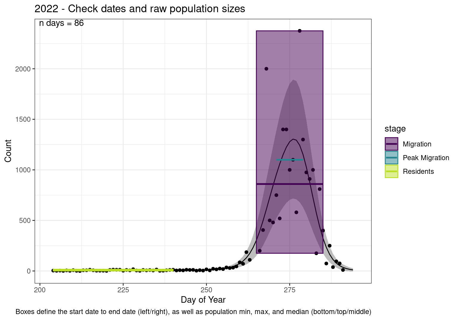
Figures
These figures are meant to be sanity checks of the models and the Resident Date cutoff (240).
Each year has two figures showing the model, one overlaid with the predicted counts (determined from the model), and one overlaid with the raw counts.
This way we could double check the calculations as well as the models.
Note that we always expect raw counts to be greater and with more variability than predicted counts. Further, I do not include the sum of counts for the raw data as this is dependent on the number of observations and somewhat misleading.
These are not particularly important plots, but we do want to have a visual of what’s going on, if only to catch mistakes in the calculations.
Interpretations
- Black line - Predicted model
- Grey ribbon - 99% CI around the model
- Yellow line (box) - Period defined as containing only residents (defined by date cutoff)
- Purple box - Period defined as migration period (defined by 5%-95% cumulative predicted counts), showing the min, max and median counts
- Blue box - Period defined as peak migration period (defined by 25%-75% cumulative predicted counts), showing the min, max and median counts
- Sum counts - Text indicating the cumulative total number of predicted counts expected in that period.
n days- the total number of days with observations for that year.
Code
for(y in unique(v$year)) {
  cat("### ", y, " {#", y, "}\n\n", sep = "")
  if(y != "2007") {
    v1 <- filter(v, year == y)
    p <- filter(pred, year == y)
    c <- filter(cum_counts, year == y)
    f <- filter(final, year == y)

    g1 <- plot_model(raw = v1, pred = p, final = f)

    pop1 <- select(f, mig_start_doy, mig_end_doy, peak_start_doy, peak_end_doy,
                   contains("pop"), -contains("ambig")) |>
      pivot_longer(everything()) |>
      mutate(type = str_extract(name, "min|max|median|mean|total|start|end"),
             stage = str_extract(name, "mig|peak|res"),
             stage = str_replace_all(stage, c("mig" = "Migration",
                                              "peak" = "Peak Migration",
                                              "res" = "Residents"))) |>
      select(-name) |>
      pivot_wider(names_from = type) |>
      mutate(start = replace_na(start, 204),
             end = replace_na(end, resident_date))

    pop2 <- pivot_longer(pop1, cols = c("start", "end"), values_to = "doy")


    g1 <- plot_model(raw = v1, pred = p, final = f) +
      geom_rect(data = pop1, aes(xmin = start, xmax = end, ymin = min, ymax = max,
                                 fill = stage, colour = stage),
                inherit.aes = FALSE) +
      geom_path(data = pop2, aes(x = doy, y = median, colour = stage), linewidth = 1) +
      geom_text(data = filter(pop1, stage != "Residents"),
                aes(x = (end - start)/2 + start, y = max, colour = stage,
                    label = paste("Sum", stage, "Counts\n", total)),
                nudge_y = c(-60, 65), nudge_x = c(-30, 0)) +
      scale_fill_viridis_d(end = 0.9, alpha = 0.5) +
      scale_colour_viridis_d(end = 0.9) +
      labs(title = paste0(y, " - Check dates and predicted population sizes"),
           caption = "Boxes define the start date to end date (left/right), as well as population min, max, and median (bottom/top/middle)\n'Total' refers to cumulative predicted observations")


    pop1 <- select(f, mig_start_doy, mig_end_doy, peak_start_doy, peak_end_doy,
                   contains("raw"), -contains("ambig")) |>
      pivot_longer(everything()) |>
      mutate(type = str_extract(name, "min|max|median|mean|total|start|end"),
             stage = str_extract(name, "mig|peak|res"),
             stage = str_replace_all(stage, c("mig" = "Migration",
                                              "peak" = "Peak Migration",
                                              "res" = "Residents"))) |>
      select(-name) |>
      pivot_wider(names_from = type) |>
      mutate(start = replace_na(start, 204),
             end = replace_na(end, resident_date))

    pop2 <- pivot_longer(pop1, cols = c("start", "end"), values_to = "doy")

    g2 <- plot_model(raw = v1, pred = p, final = f) +
      geom_rect(data = pop1, aes(xmin = start, xmax = end, ymin = min, ymax = max,
                                 fill = stage, colour = stage),
                inherit.aes = FALSE) +
      geom_path(data = pop2, aes(x = doy, y = median, colour = stage), linewidth = 1) +
      scale_fill_viridis_d(end = 0.9, alpha = 0.5) +
      scale_colour_viridis_d(end = 0.9) +
      labs(title = paste0(y, " - Check dates and raw population sizes"),
           caption = "Boxes define the start date to end date (left/right), as well as population min, max, and median (bottom/top/middle)")

    cat(":::{.panel-tabset}\n\n")
    cat("#### Predicted Counts\n\n")
    print(g1)
    cat("\n\n")
    cat("#### Raw Counts\n\n")
    print(g2)
    cat("\n\n")
    cat(":::\n\n")

    cat("\n\n")

  } else cat("No Data for 2007\n\n")
}
1999
Warning: Removed 1 row containing missing values or values outside the scale range
(`geom_rect()`).
Warning: Removed 1 row containing missing values or values outside the scale range
(`geom_text()`).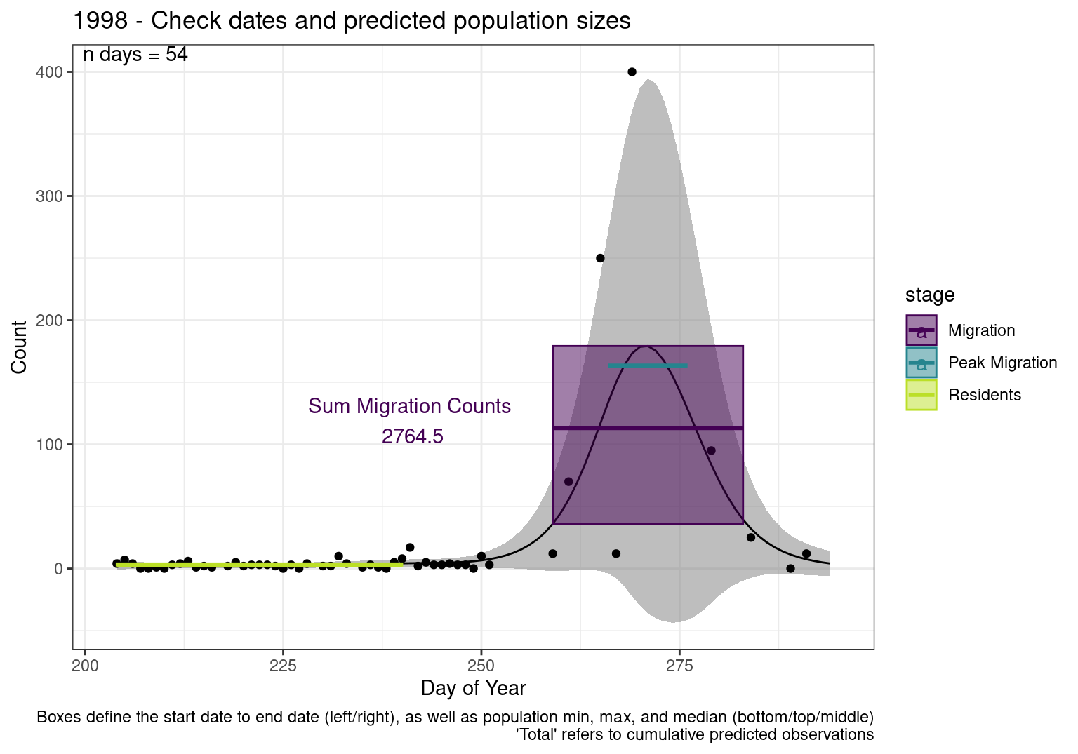
Warning: Removed 1 row containing missing values or values outside the scale range
(`geom_rect()`).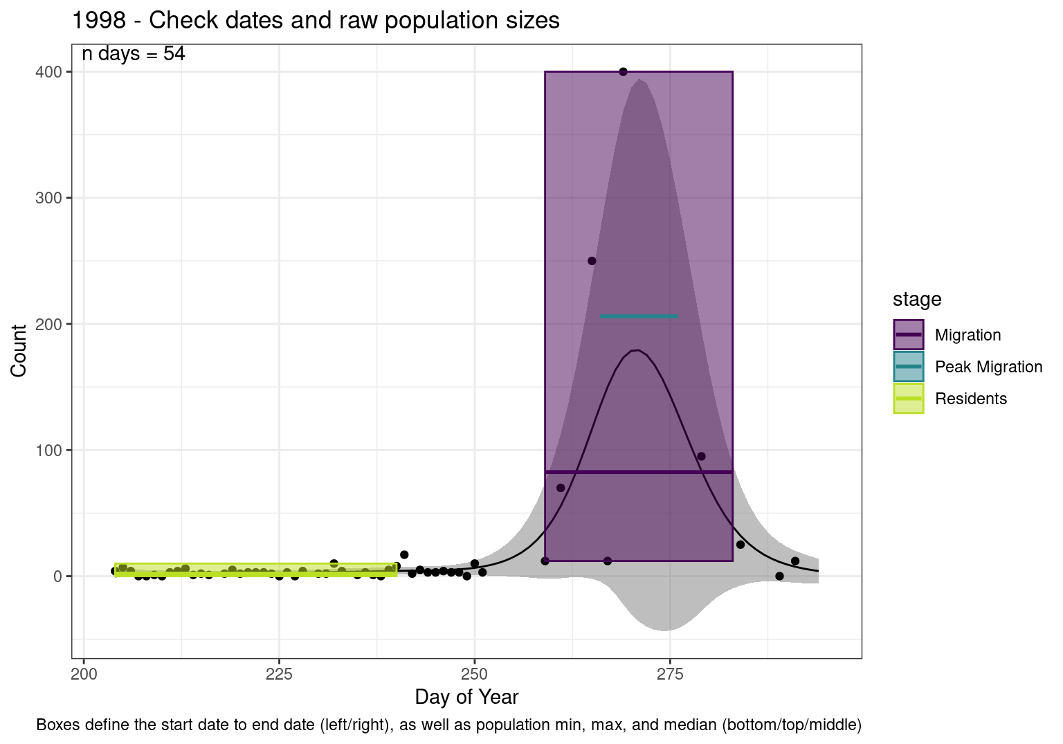
2000
Warning: Removed 1 row containing missing values or values outside the scale range
(`geom_rect()`).
Removed 1 row containing missing values or values outside the scale range
(`geom_text()`).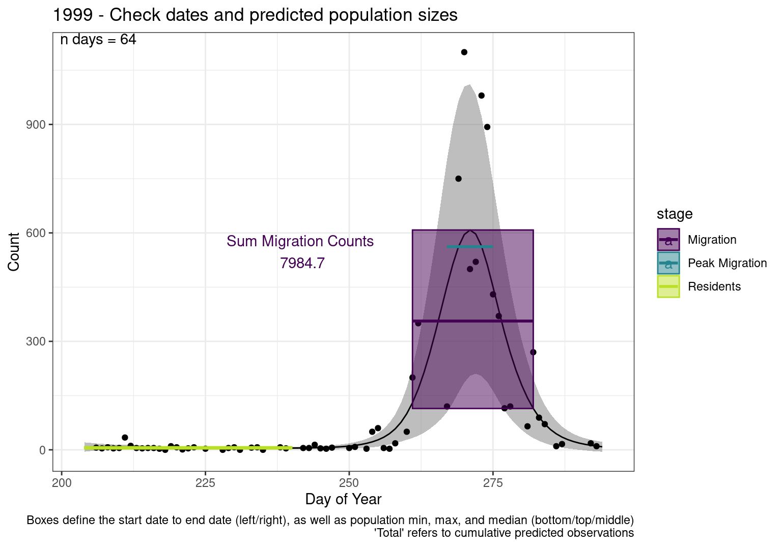
Warning: Removed 1 row containing missing values or values outside the scale range
(`geom_rect()`).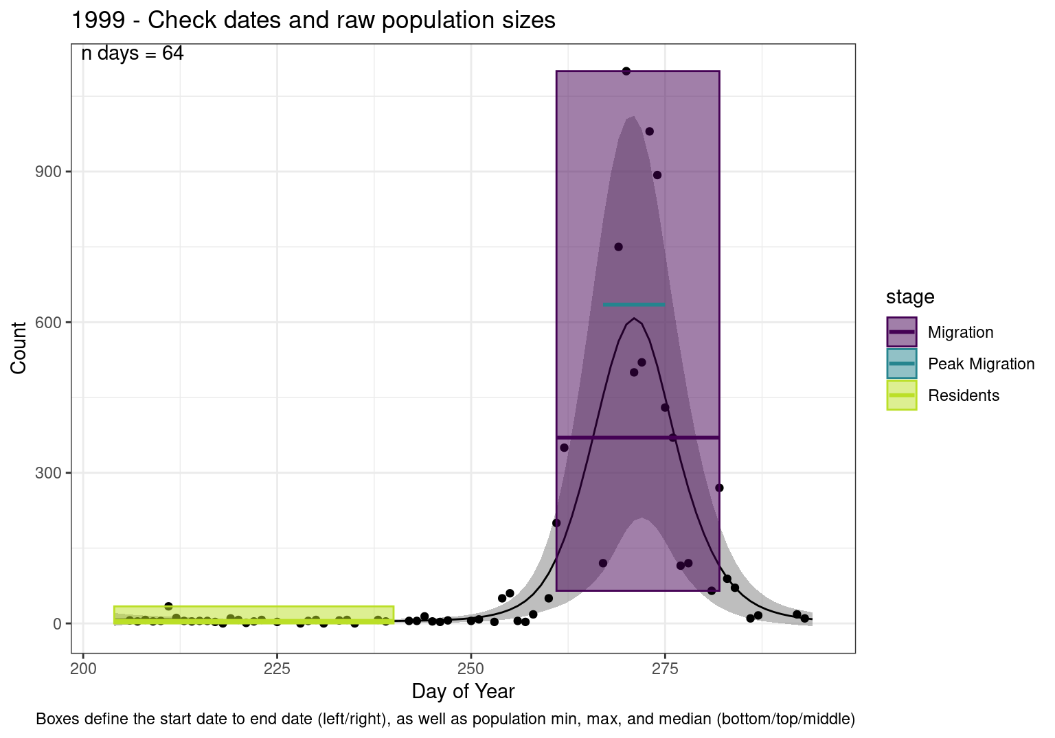
2001
Warning: Removed 1 row containing missing values or values outside the scale range
(`geom_rect()`).
Removed 1 row containing missing values or values outside the scale range
(`geom_text()`).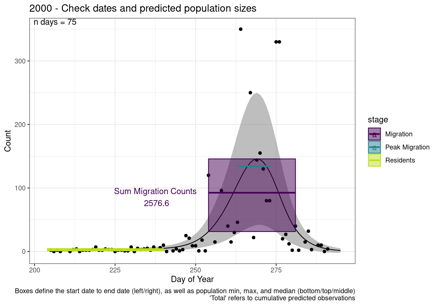
Warning: Removed 1 row containing missing values or values outside the scale range
(`geom_rect()`).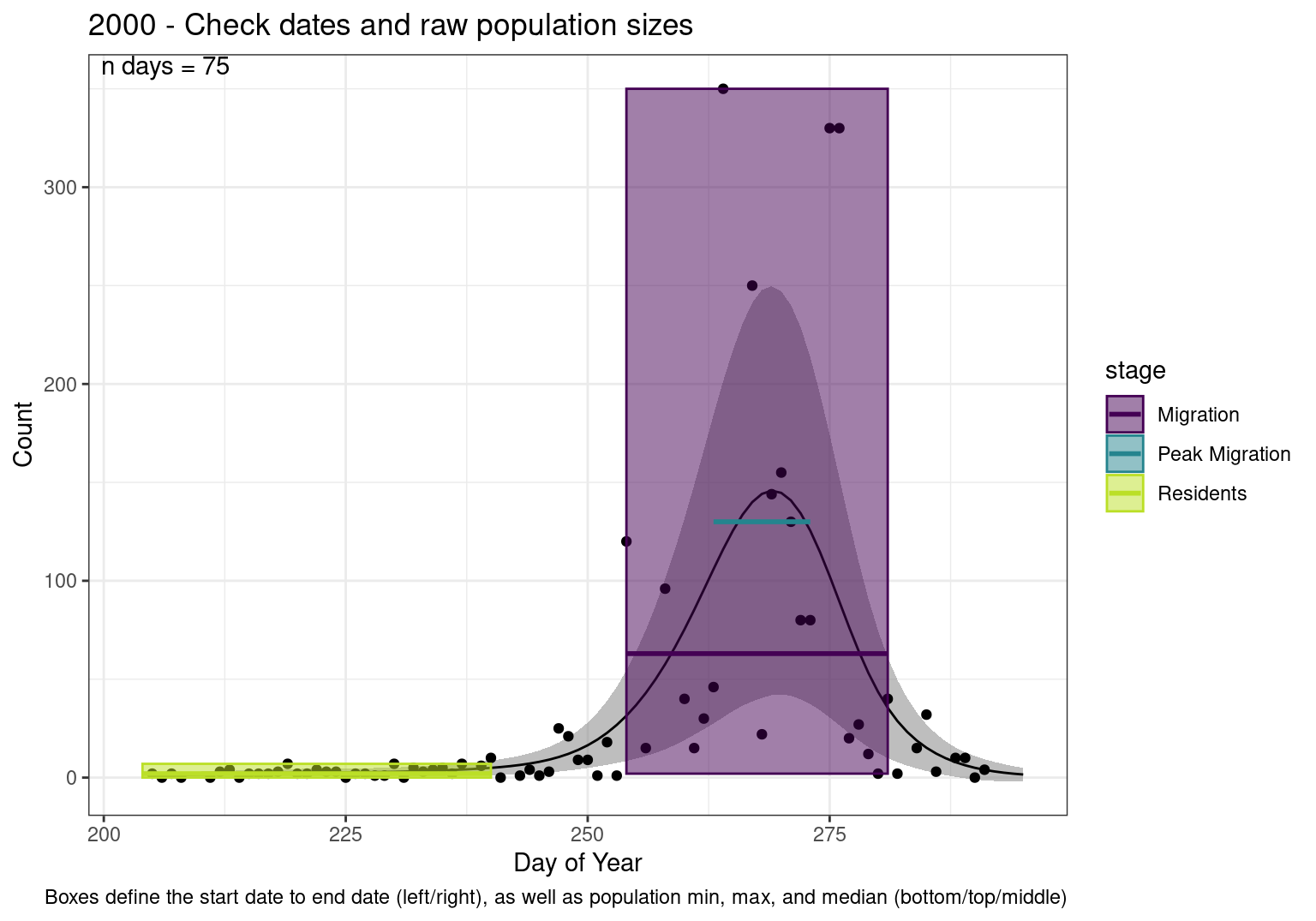
2002
Warning: Removed 1 row containing missing values or values outside the scale range
(`geom_rect()`).
Removed 1 row containing missing values or values outside the scale range
(`geom_text()`).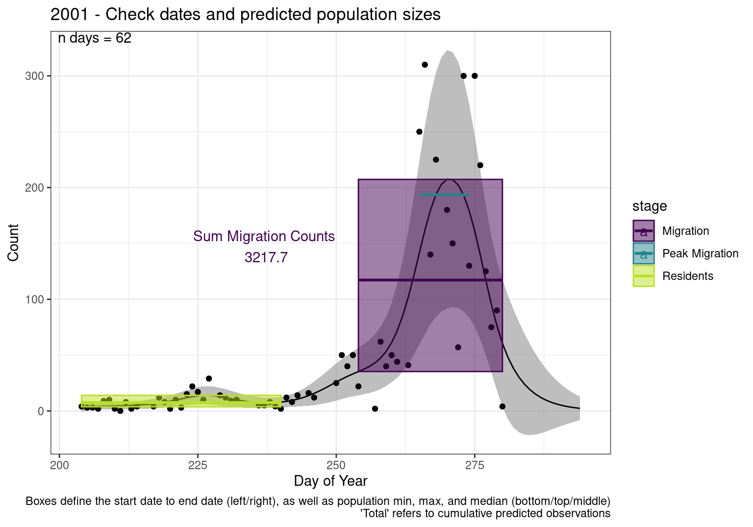
Warning: Removed 1 row containing missing values or values outside the scale range
(`geom_rect()`).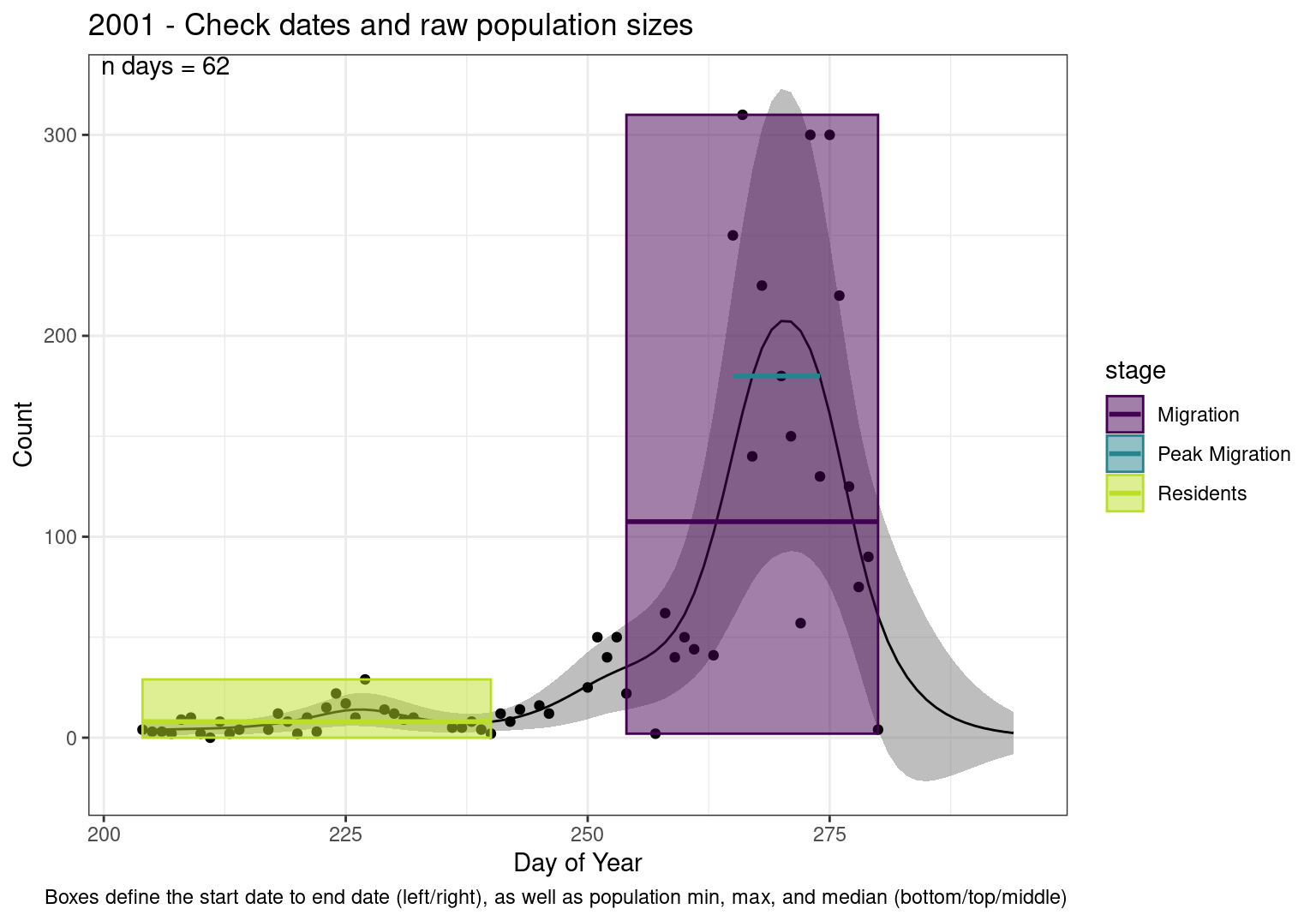
2003
Warning: Removed 1 row containing missing values or values outside the scale range
(`geom_rect()`).
Removed 1 row containing missing values or values outside the scale range
(`geom_text()`).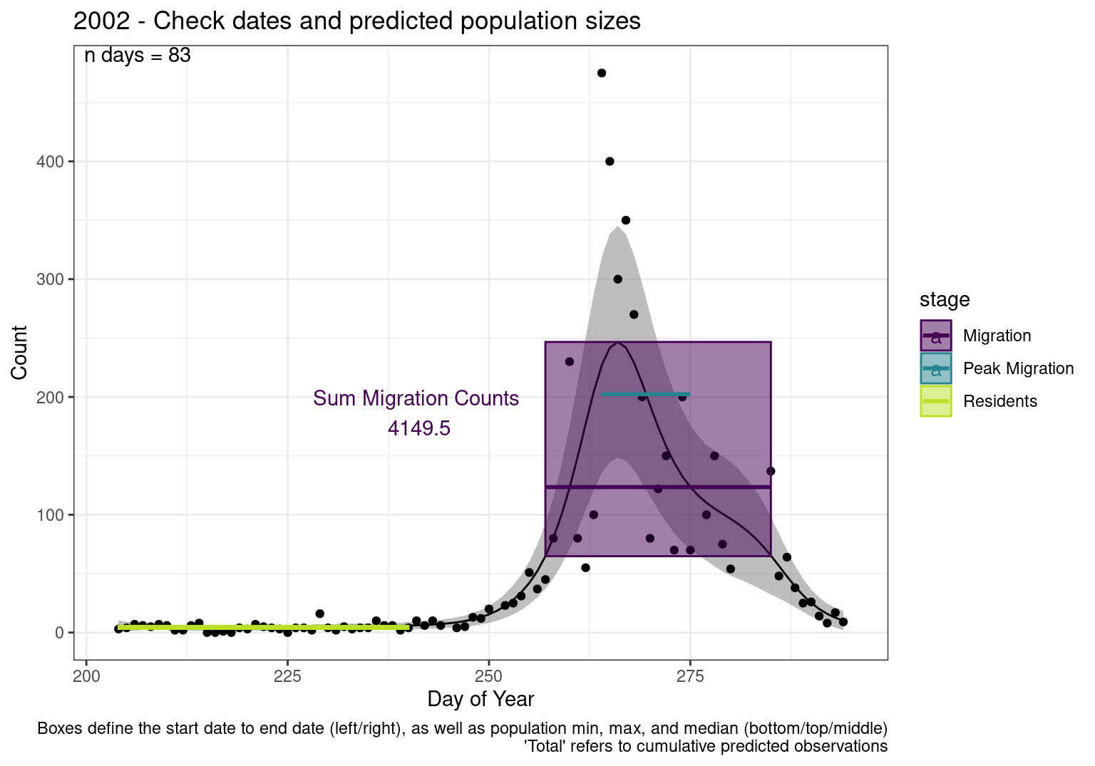
Warning: Removed 1 row containing missing values or values outside the scale range
(`geom_rect()`).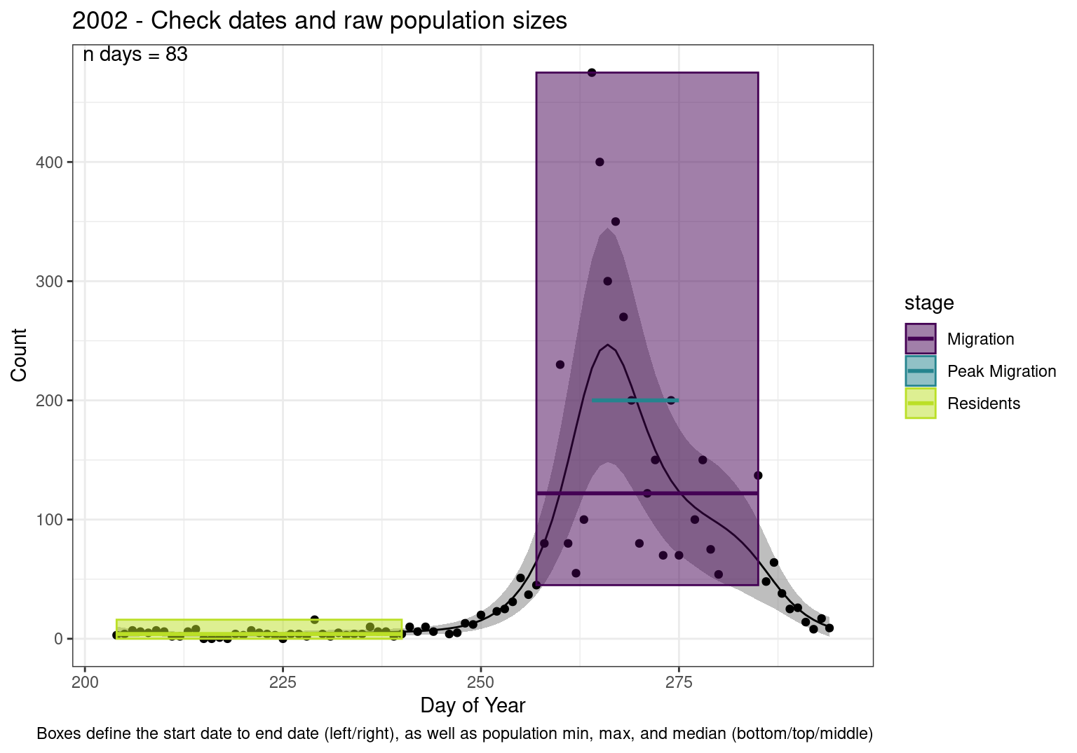
2004
Warning: Removed 1 row containing missing values or values outside the scale range
(`geom_rect()`).
Removed 1 row containing missing values or values outside the scale range
(`geom_text()`).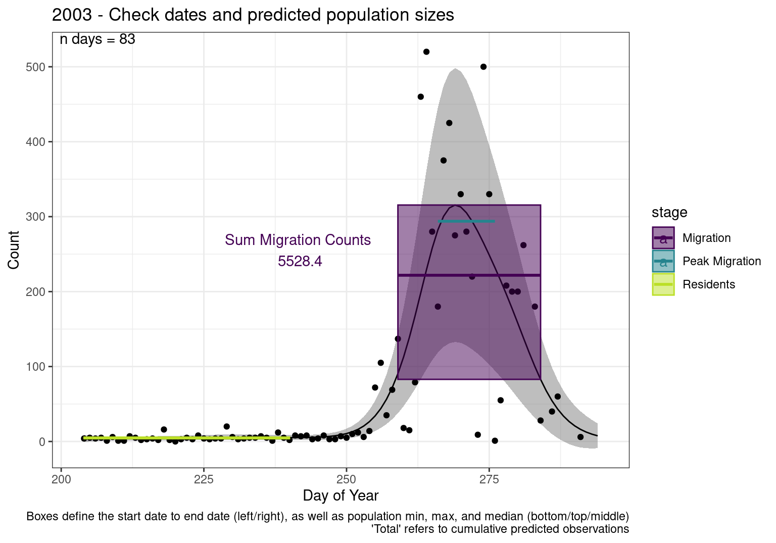
Warning: Removed 1 row containing missing values or values outside the scale range
(`geom_rect()`).
2005
Warning: Removed 1 row containing missing values or values outside the scale range
(`geom_rect()`).
Removed 1 row containing missing values or values outside the scale range
(`geom_text()`).
Warning: Removed 1 row containing missing values or values outside the scale range
(`geom_rect()`).
2006
Warning: Removed 1 row containing missing values or values outside the scale range
(`geom_rect()`).
Removed 1 row containing missing values or values outside the scale range
(`geom_text()`).
Warning: Removed 1 row containing missing values or values outside the scale range
(`geom_rect()`).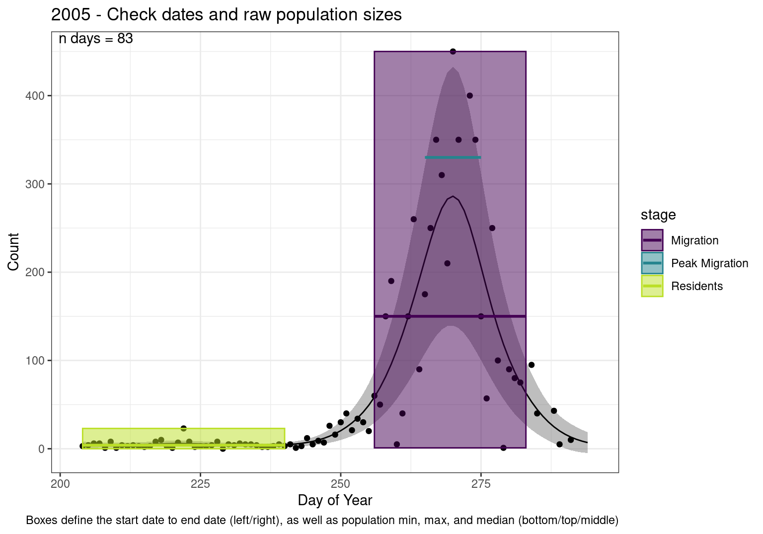
2007
No Data for 2007
2008
Warning: Removed 1 row containing missing values or values outside the scale range
(`geom_rect()`).
Removed 1 row containing missing values or values outside the scale range
(`geom_text()`).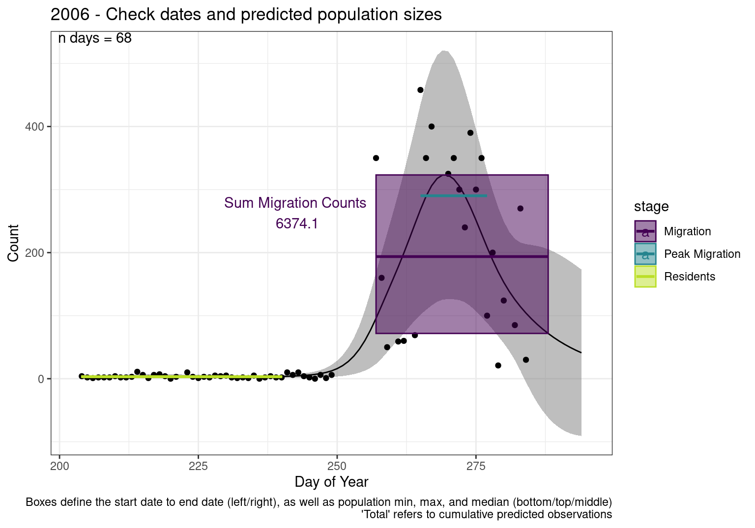
Warning: Removed 1 row containing missing values or values outside the scale range
(`geom_rect()`).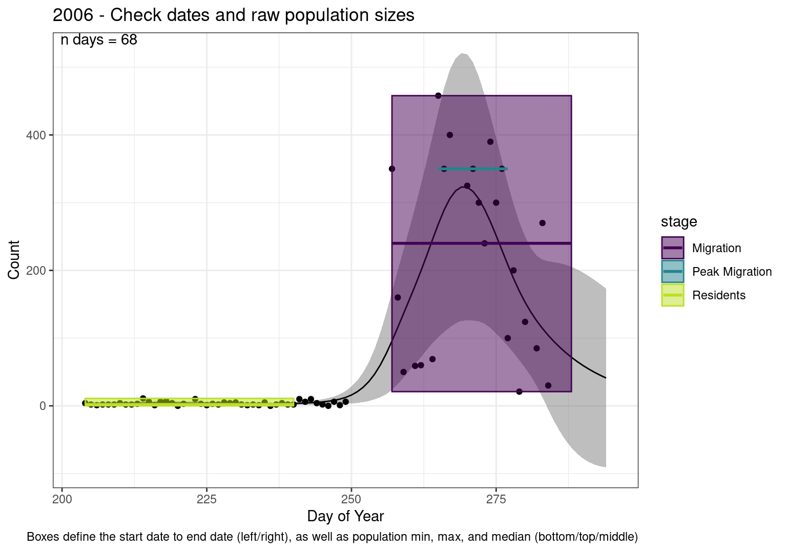
2009
Warning: Removed 1 row containing missing values or values outside the scale range
(`geom_rect()`).
Removed 1 row containing missing values or values outside the scale range
(`geom_text()`).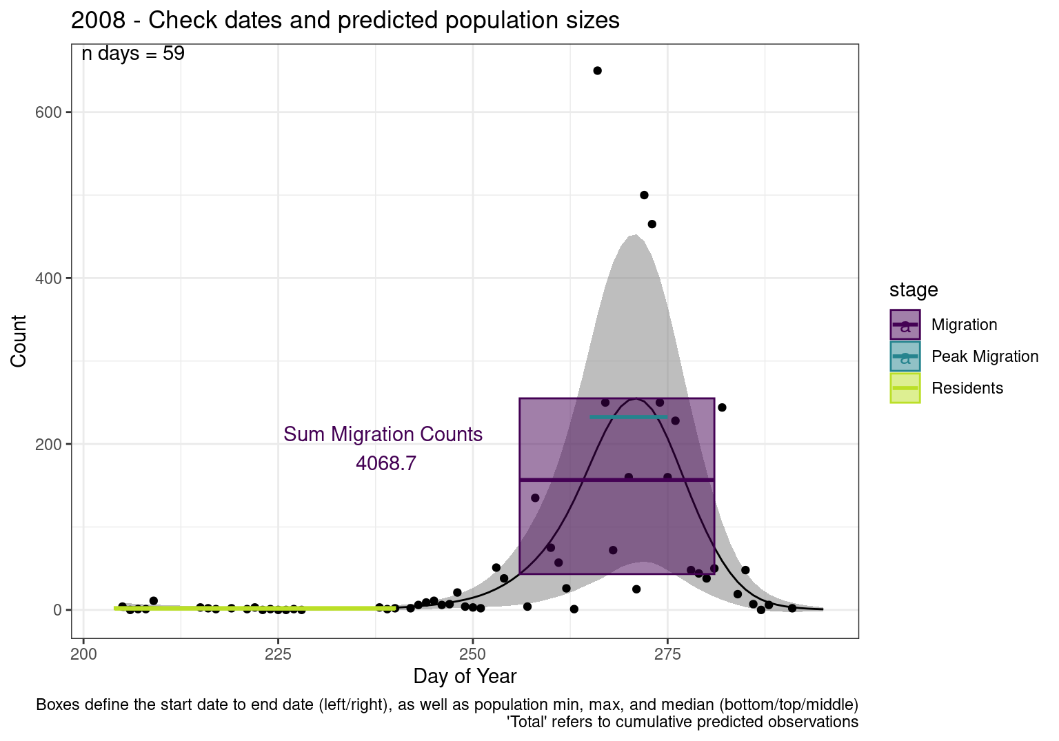
Warning: Removed 1 row containing missing values or values outside the scale range
(`geom_rect()`).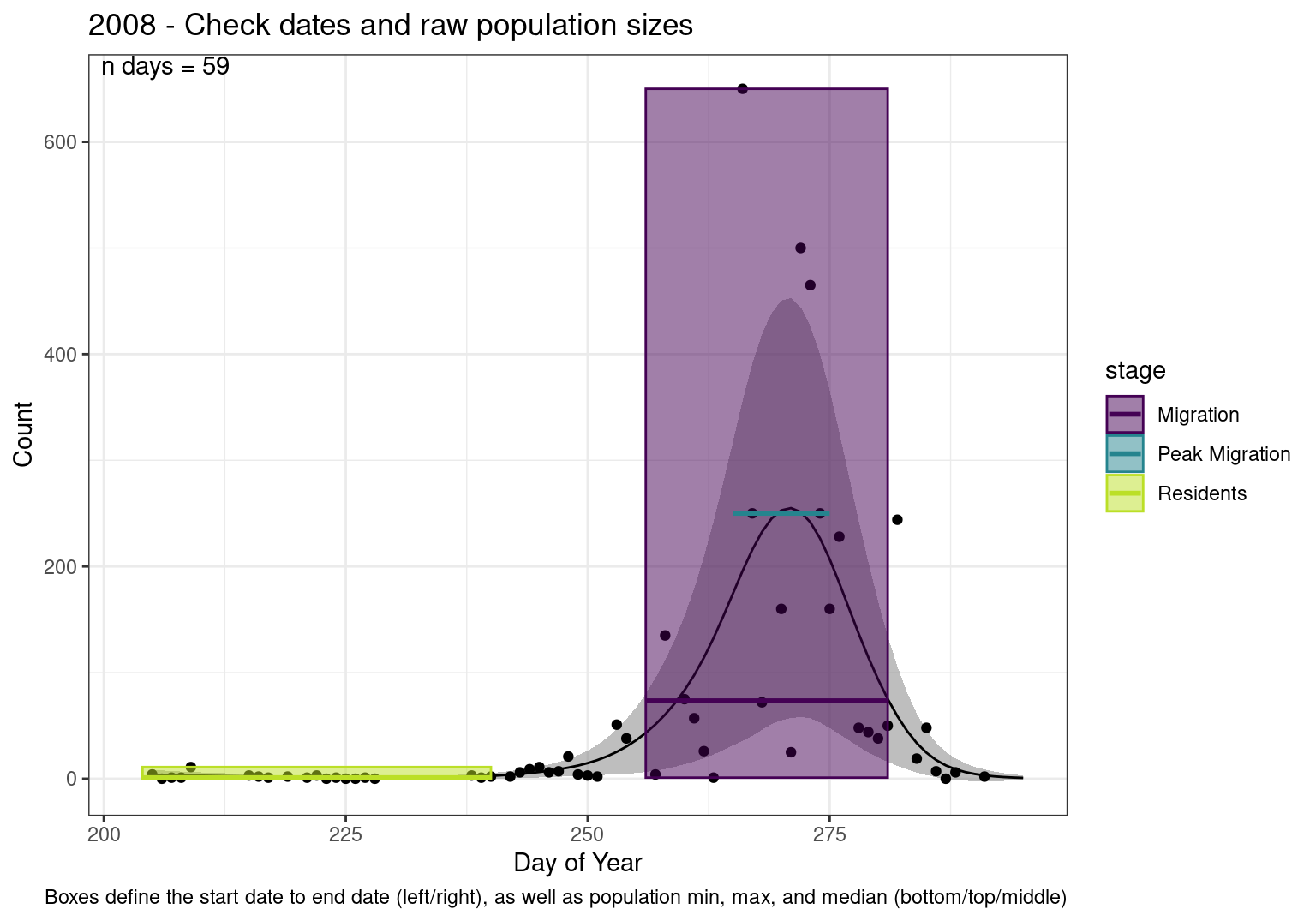
2010
Warning: Removed 1 row containing missing values or values outside the scale range
(`geom_rect()`).
Removed 1 row containing missing values or values outside the scale range
(`geom_text()`).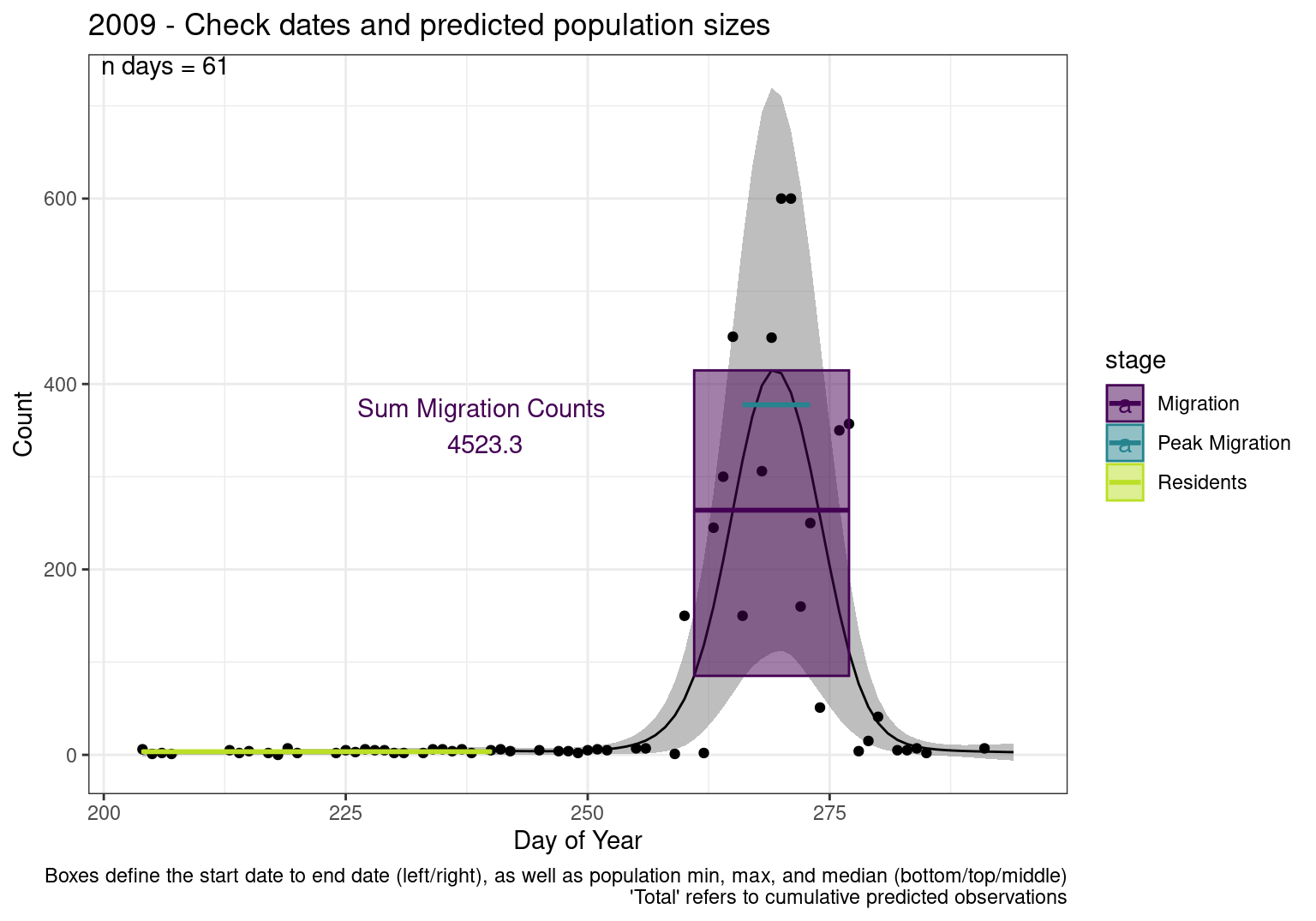
Warning: Removed 1 row containing missing values or values outside the scale range
(`geom_rect()`).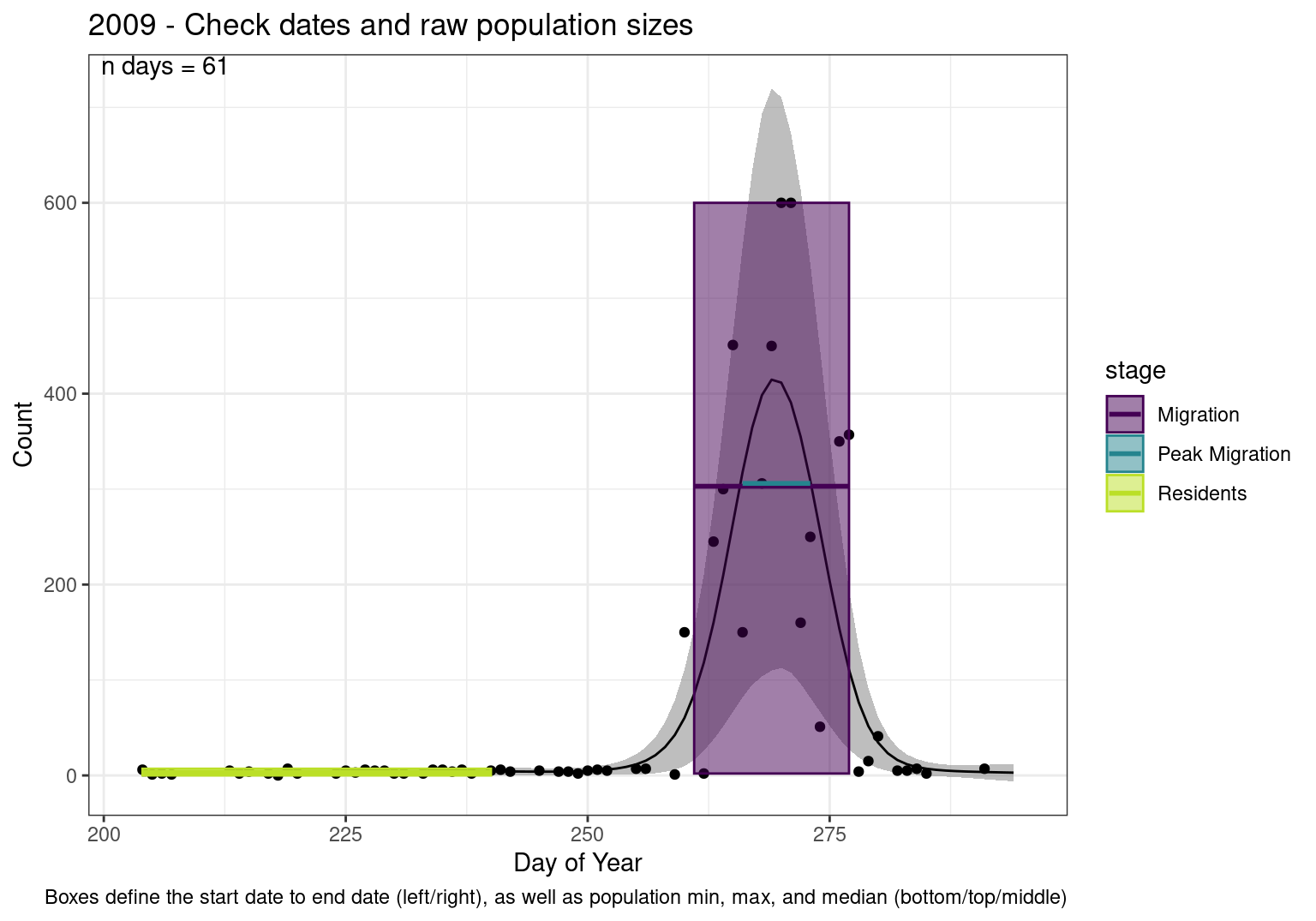
2011
Warning: Removed 1 row containing missing values or values outside the scale range
(`geom_rect()`).
Removed 1 row containing missing values or values outside the scale range
(`geom_text()`).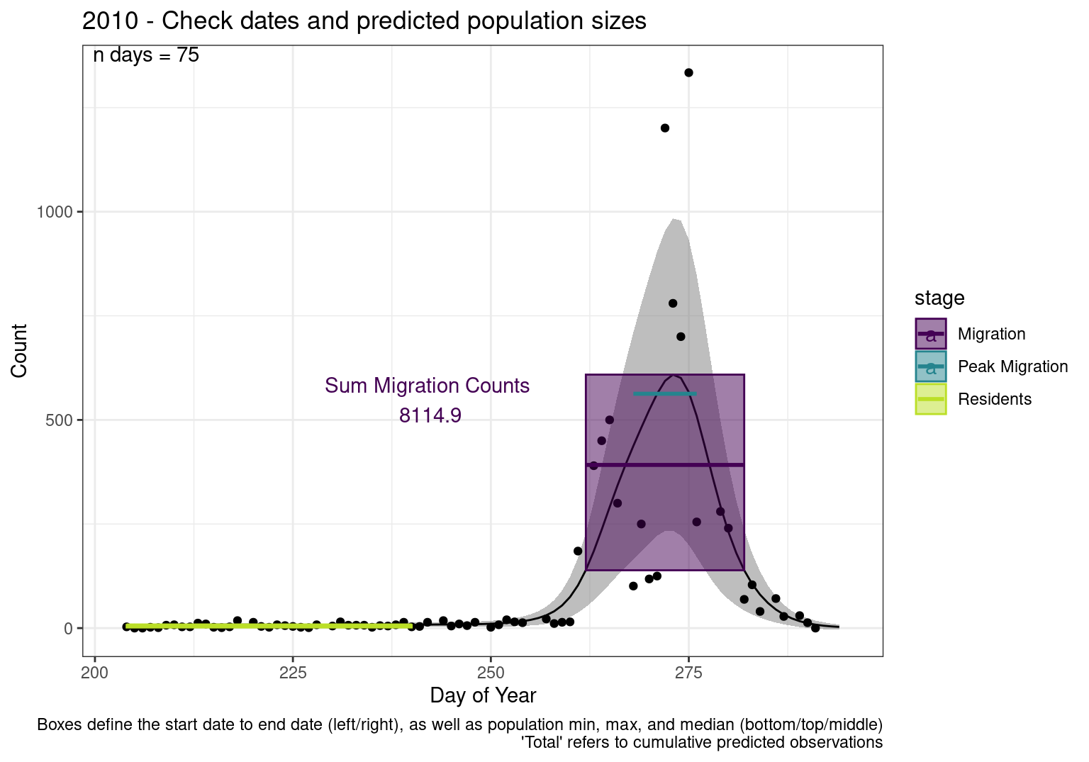
Warning: Removed 1 row containing missing values or values outside the scale range
(`geom_rect()`).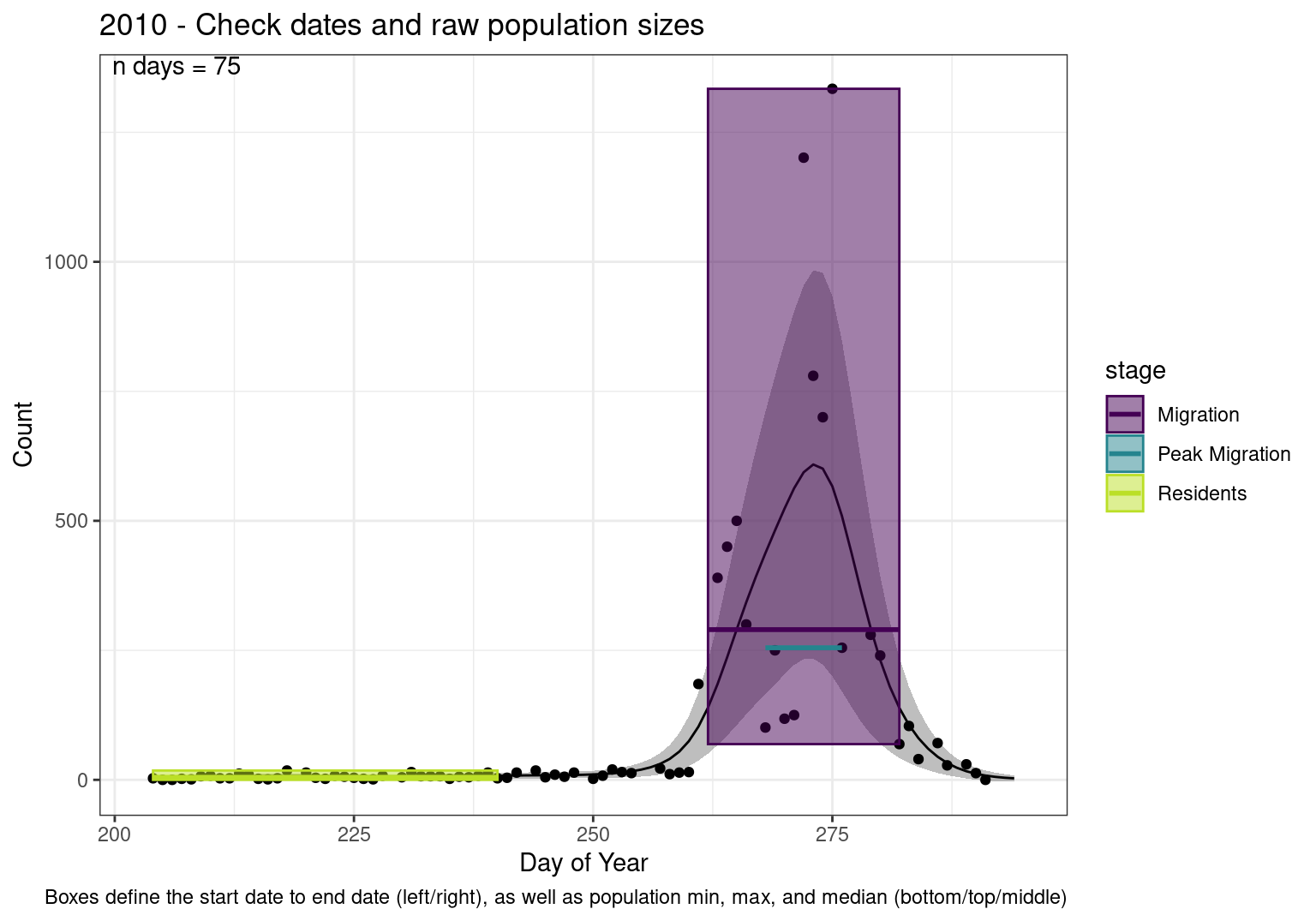
2012
Warning: Removed 1 row containing missing values or values outside the scale range
(`geom_rect()`).
Removed 1 row containing missing values or values outside the scale range
(`geom_text()`).
Warning: Removed 1 row containing missing values or values outside the scale range
(`geom_rect()`).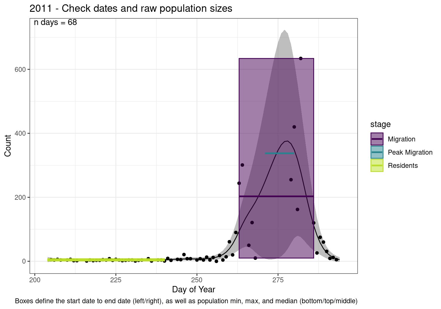
2013
Warning: Removed 1 row containing missing values or values outside the scale range
(`geom_rect()`).
Removed 1 row containing missing values or values outside the scale range
(`geom_text()`).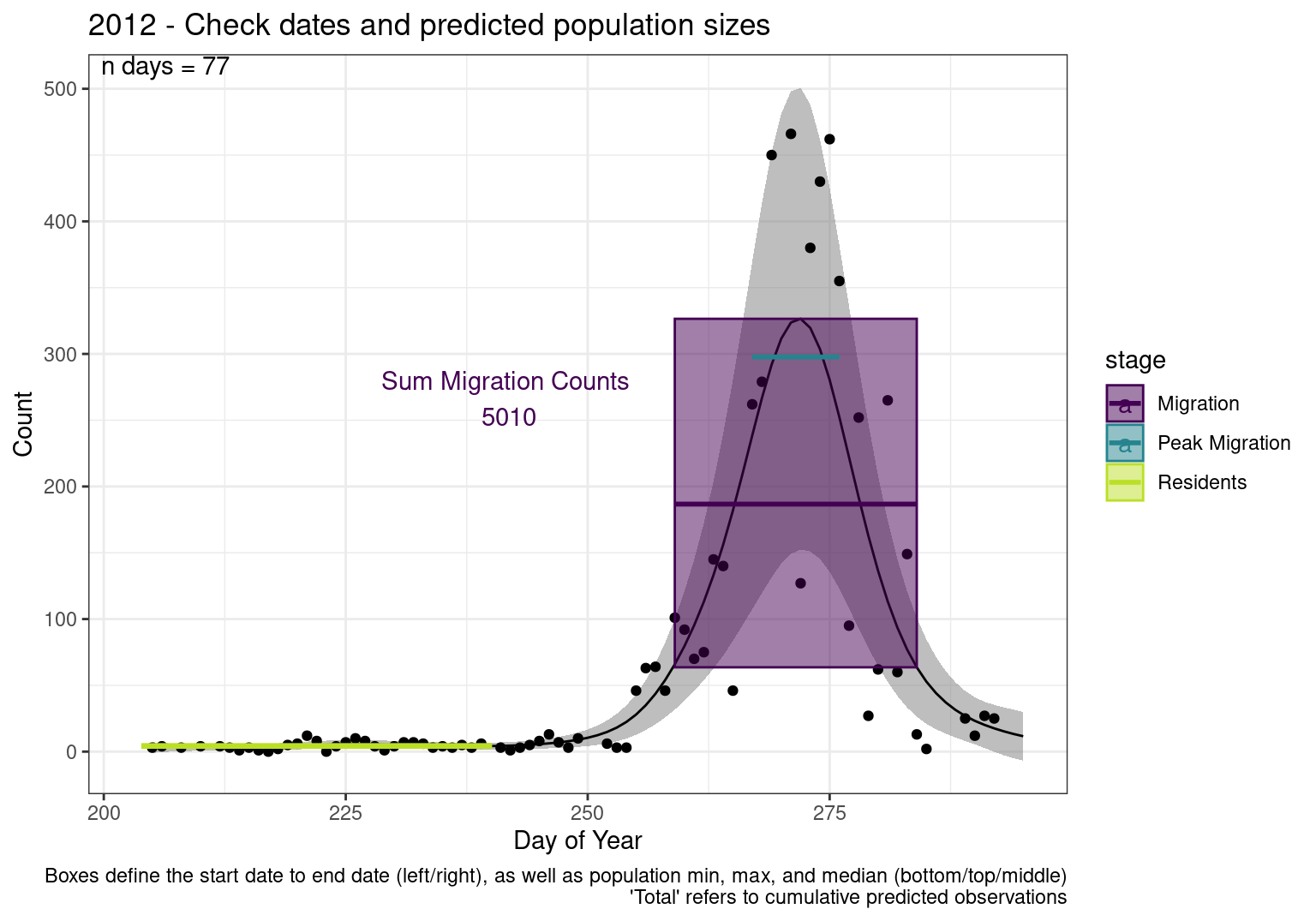
Warning: Removed 1 row containing missing values or values outside the scale range
(`geom_rect()`).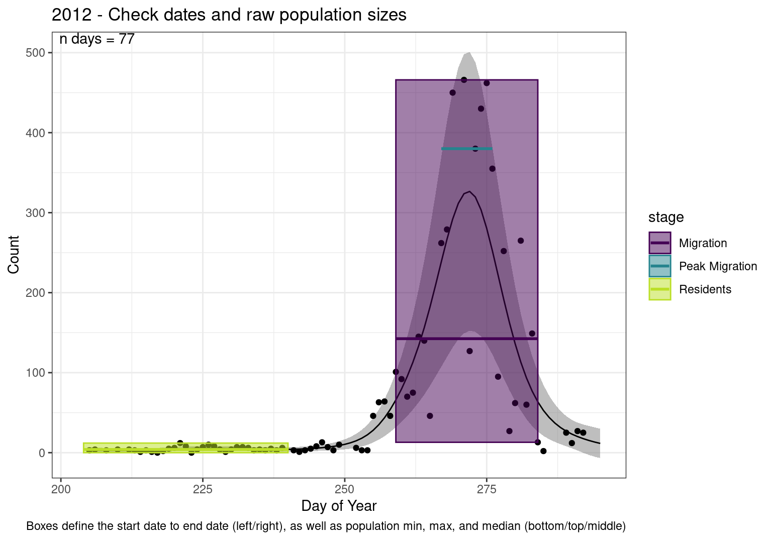
2014
Warning: Removed 1 row containing missing values or values outside the scale range
(`geom_rect()`).
Removed 1 row containing missing values or values outside the scale range
(`geom_text()`).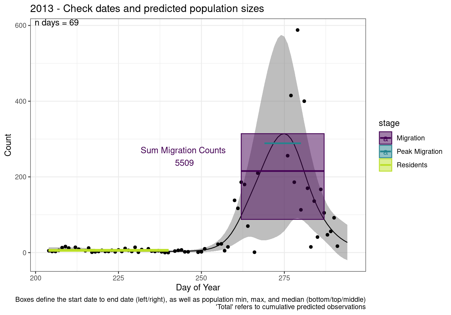
Warning: Removed 1 row containing missing values or values outside the scale range
(`geom_rect()`).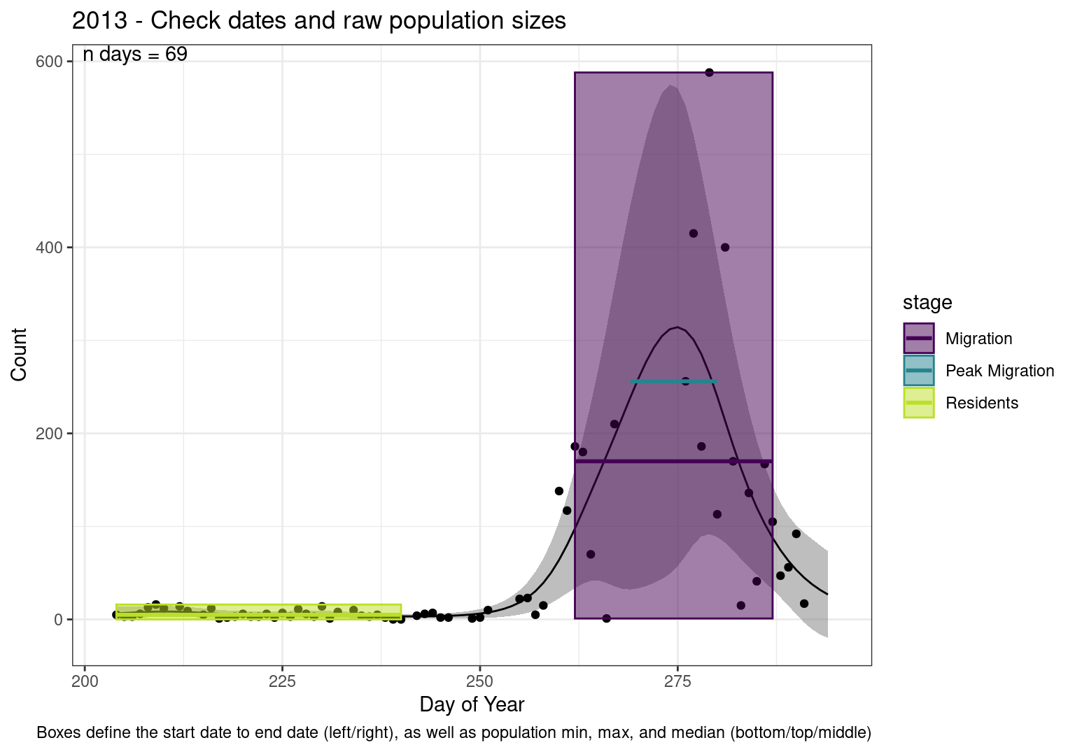
2015
Warning: Removed 1 row containing missing values or values outside the scale range
(`geom_rect()`).
Removed 1 row containing missing values or values outside the scale range
(`geom_text()`).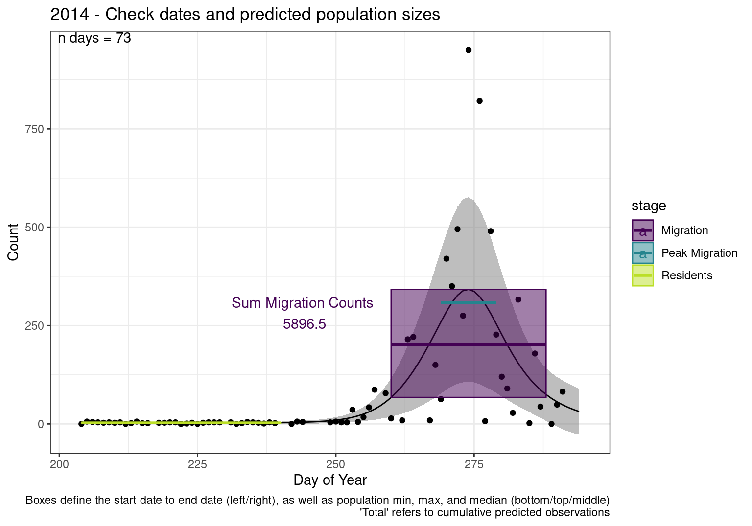
Warning: Removed 1 row containing missing values or values outside the scale range
(`geom_rect()`).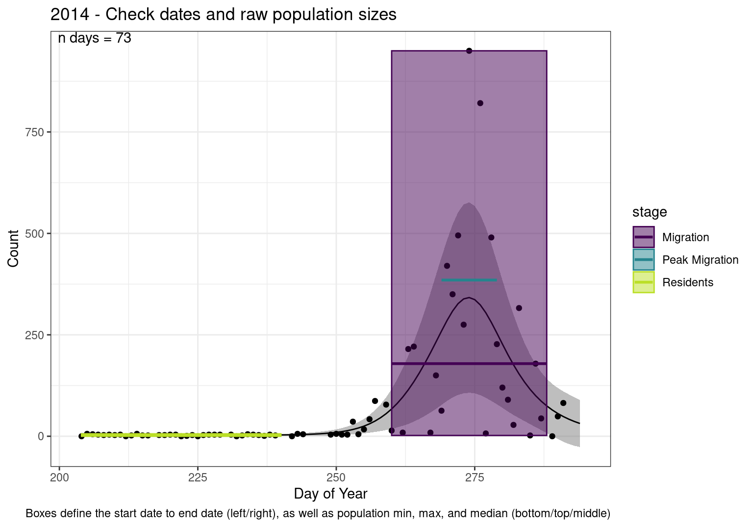
2016
Warning: Removed 1 row containing missing values or values outside the scale range
(`geom_rect()`).
Removed 1 row containing missing values or values outside the scale range
(`geom_text()`).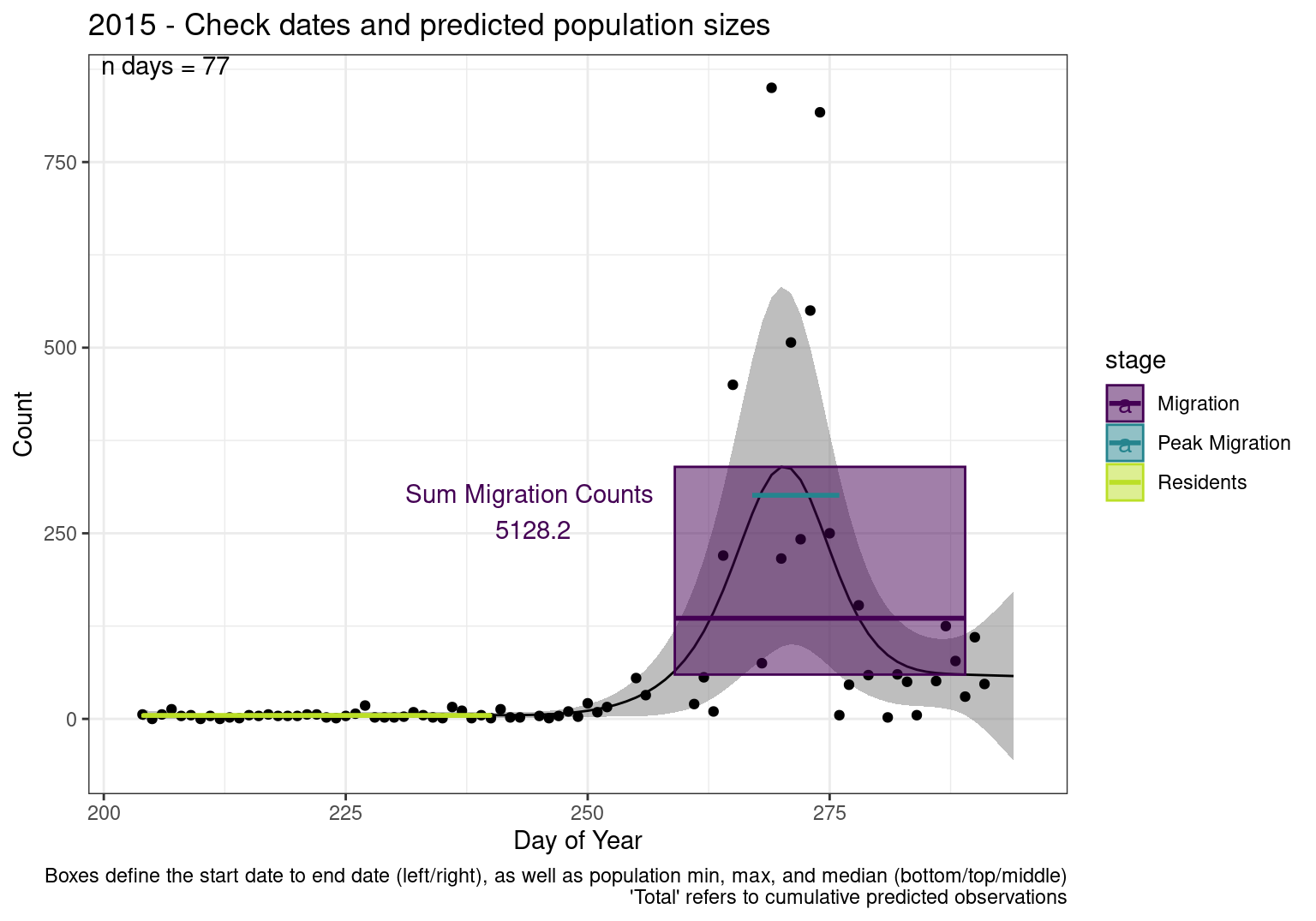
Warning: Removed 1 row containing missing values or values outside the scale range
(`geom_rect()`).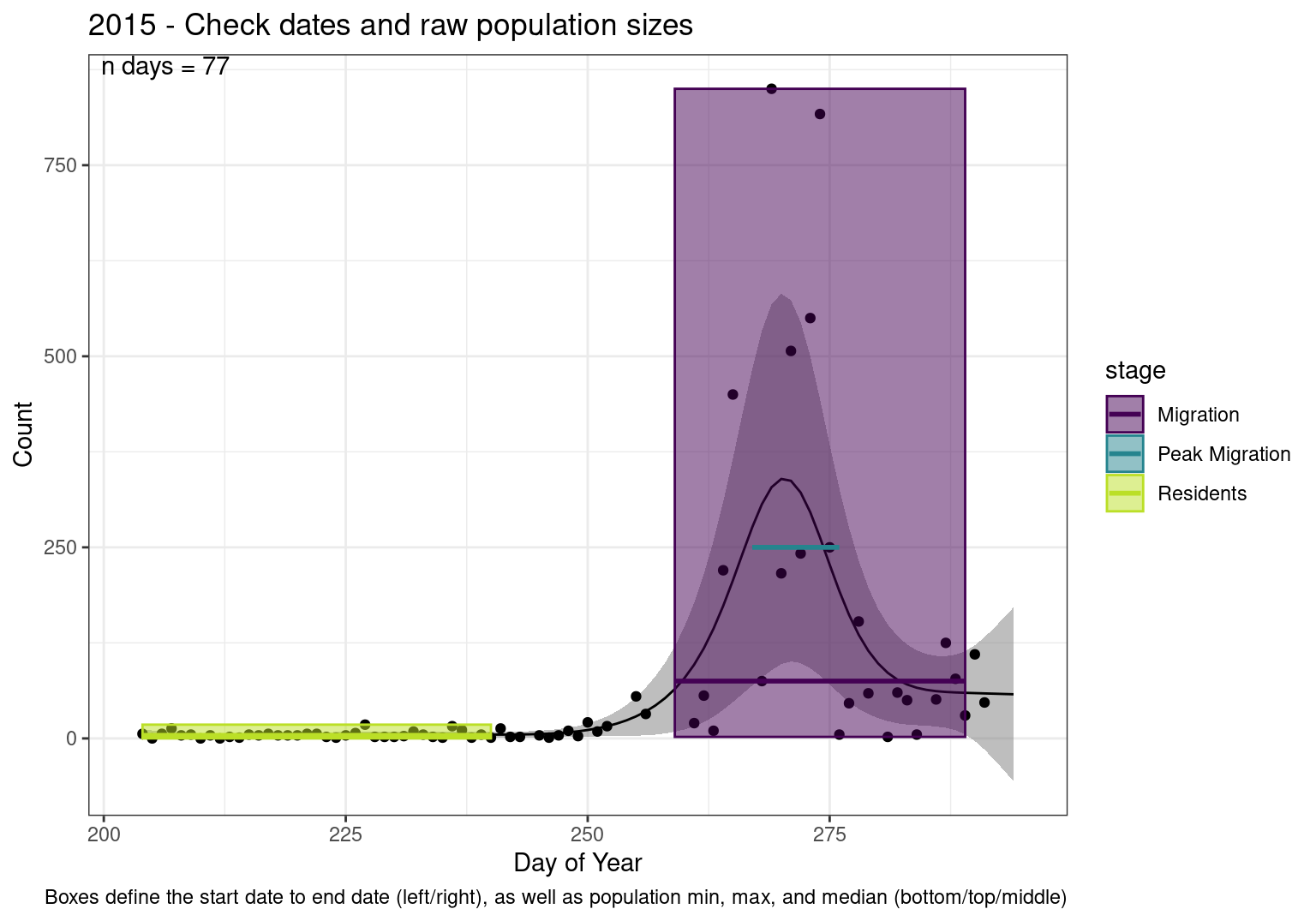
2017
Warning: Removed 1 row containing missing values or values outside the scale range
(`geom_rect()`).
Removed 1 row containing missing values or values outside the scale range
(`geom_text()`).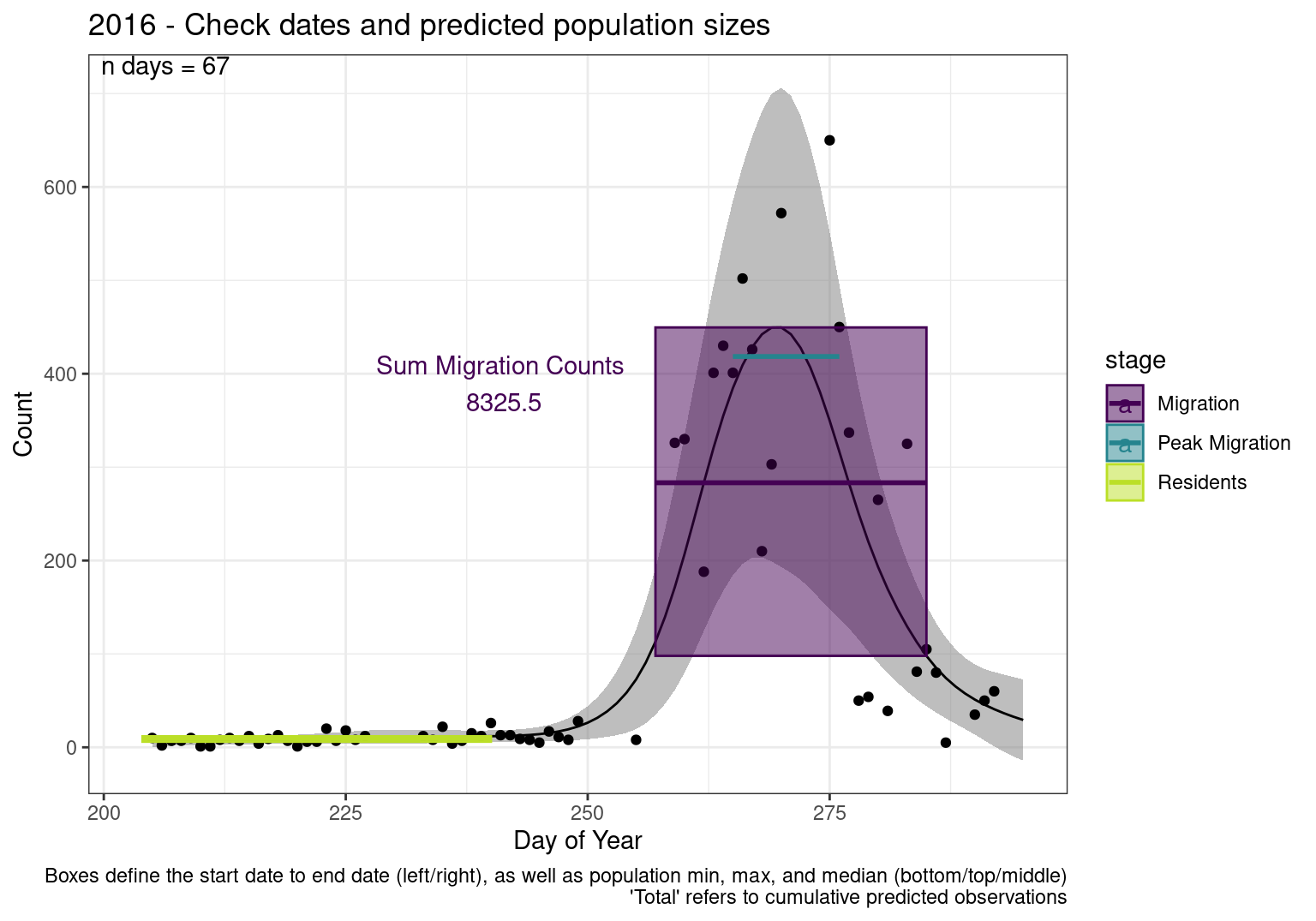
Warning: Removed 1 row containing missing values or values outside the scale range
(`geom_rect()`).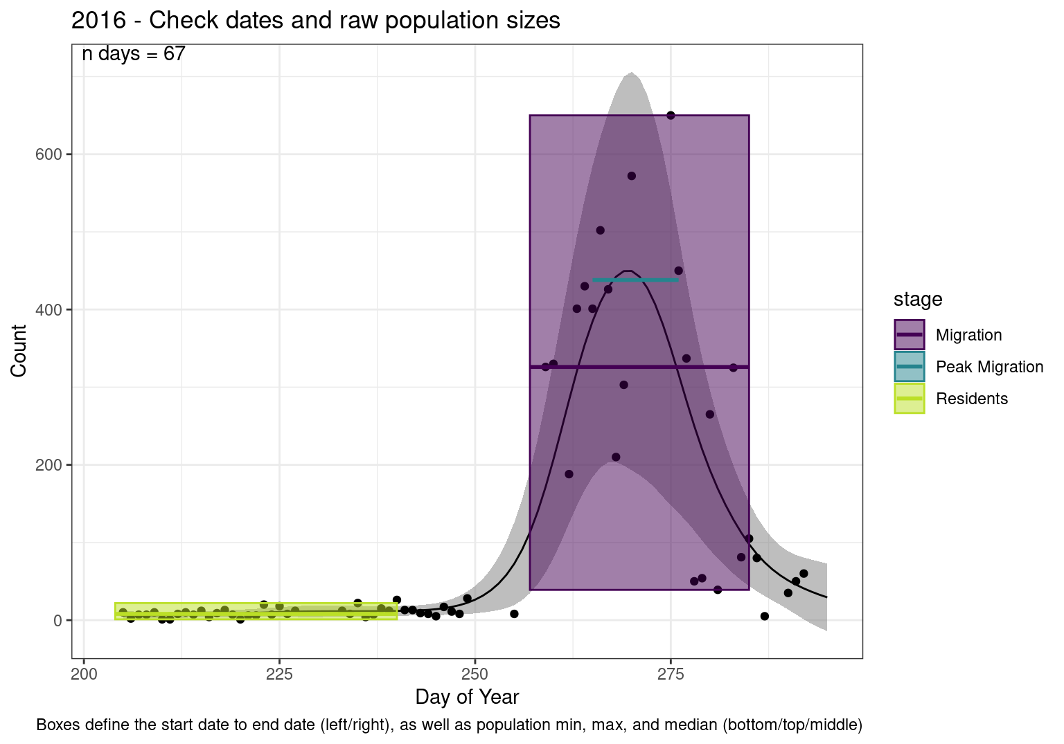
2018
Warning: Removed 1 row containing missing values or values outside the scale range
(`geom_rect()`).
Removed 1 row containing missing values or values outside the scale range
(`geom_text()`).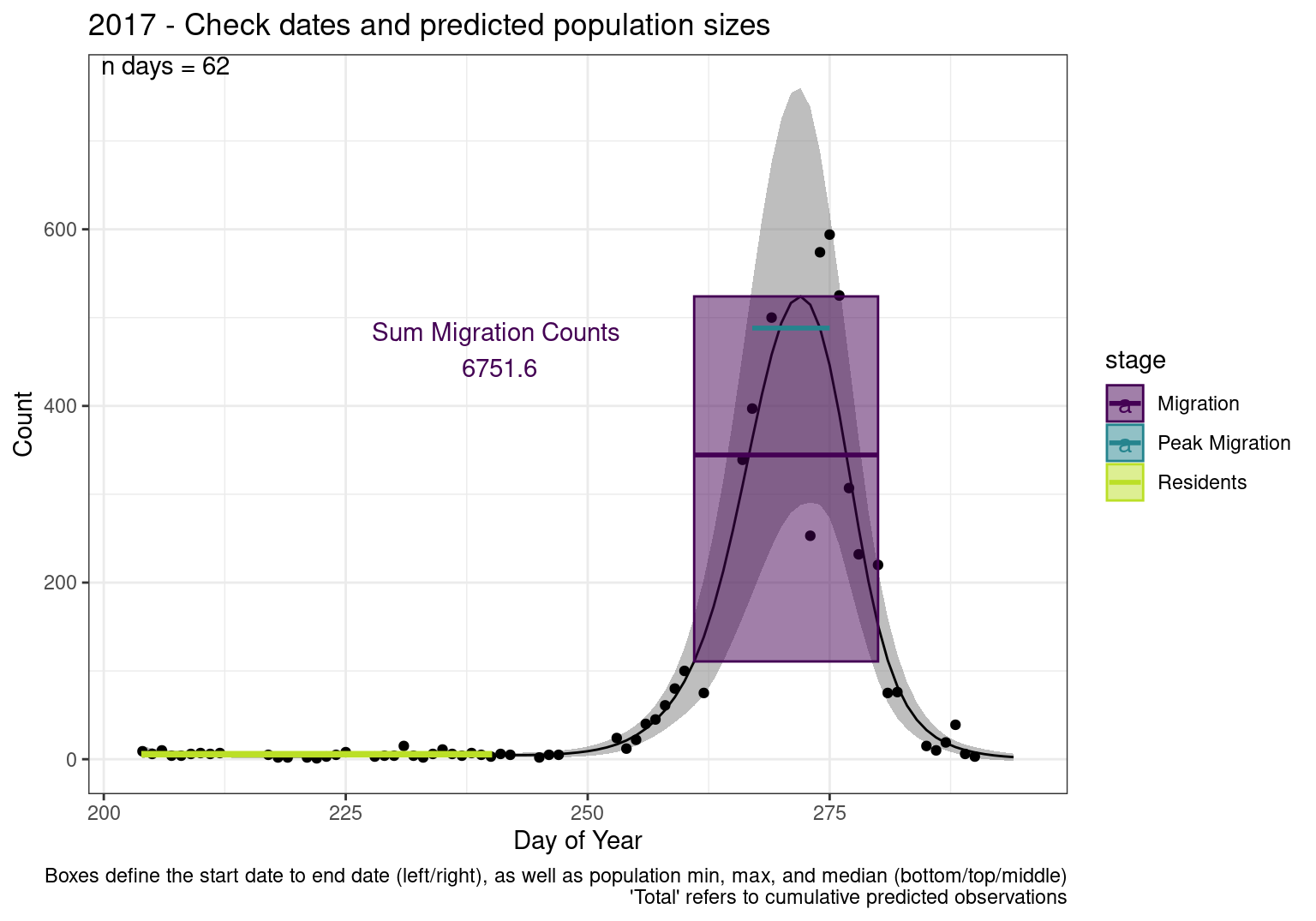
Warning: Removed 1 row containing missing values or values outside the scale range
(`geom_rect()`).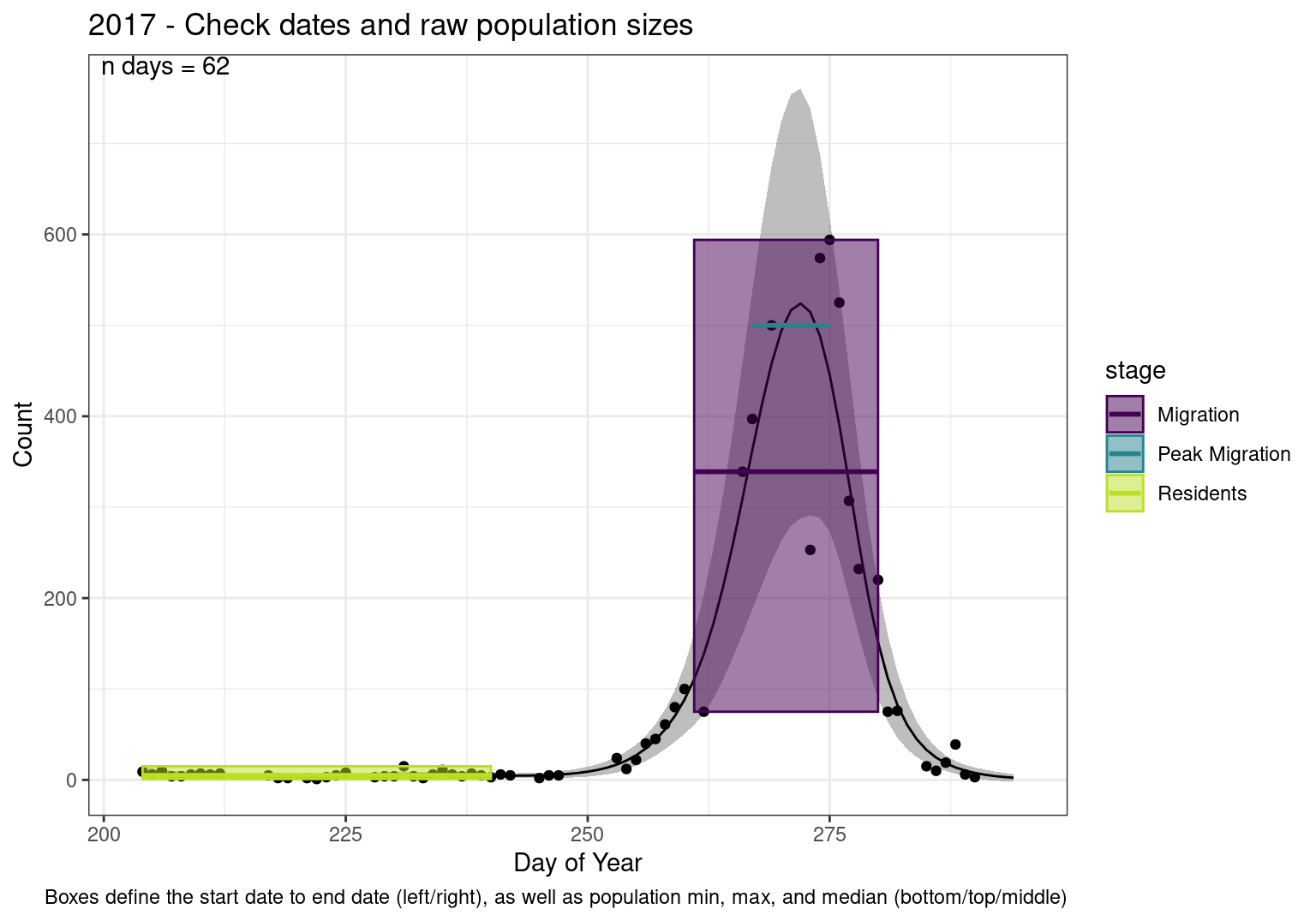
2019
Warning: Removed 1 row containing missing values or values outside the scale range
(`geom_rect()`).
Removed 1 row containing missing values or values outside the scale range
(`geom_text()`).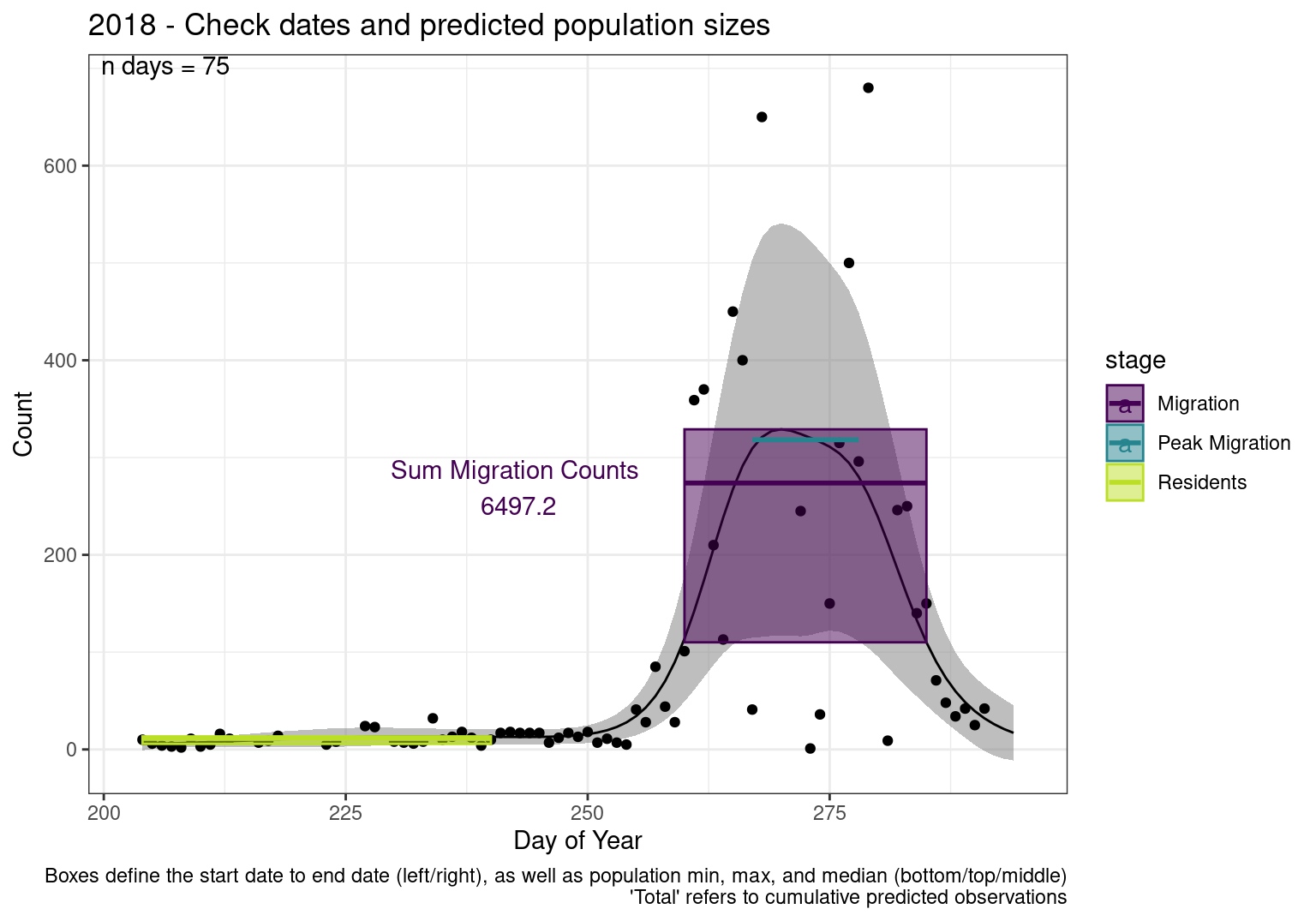
Warning: Removed 1 row containing missing values or values outside the scale range
(`geom_rect()`).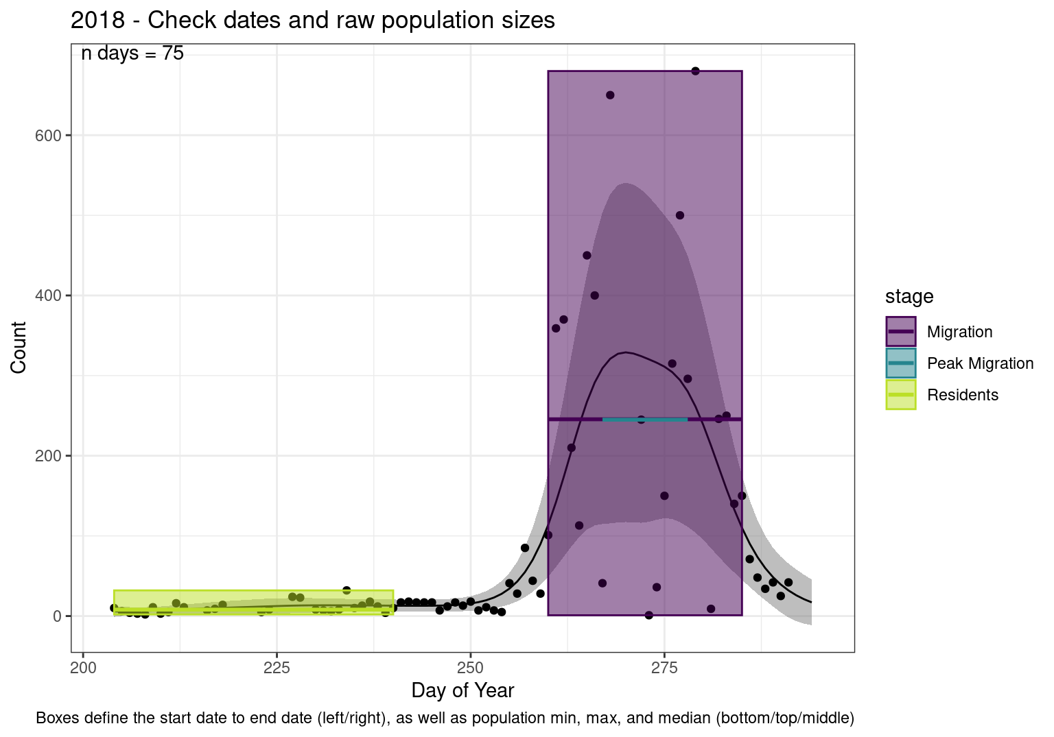
2020
Warning: Removed 1 row containing missing values or values outside the scale range
(`geom_rect()`).
Removed 1 row containing missing values or values outside the scale range
(`geom_text()`).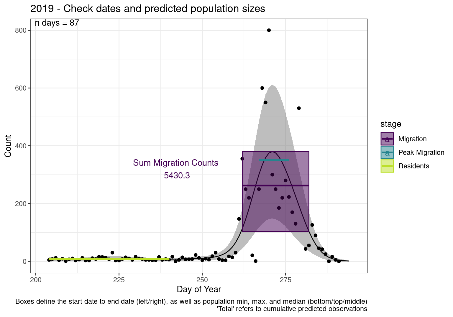
Warning: Removed 1 row containing missing values or values outside the scale range
(`geom_rect()`).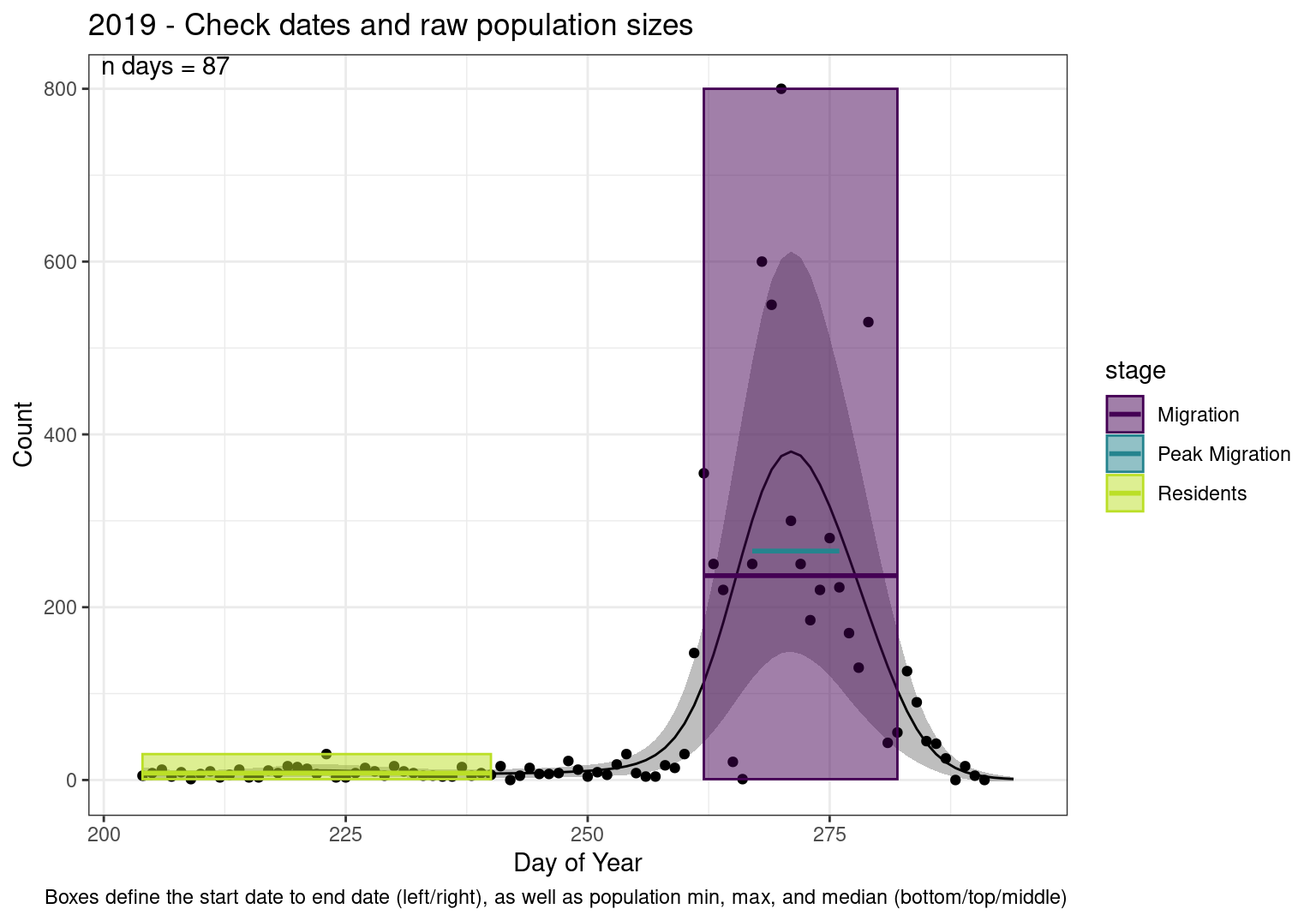
2021
Warning: Removed 1 row containing missing values or values outside the scale range
(`geom_rect()`).
Removed 1 row containing missing values or values outside the scale range
(`geom_text()`).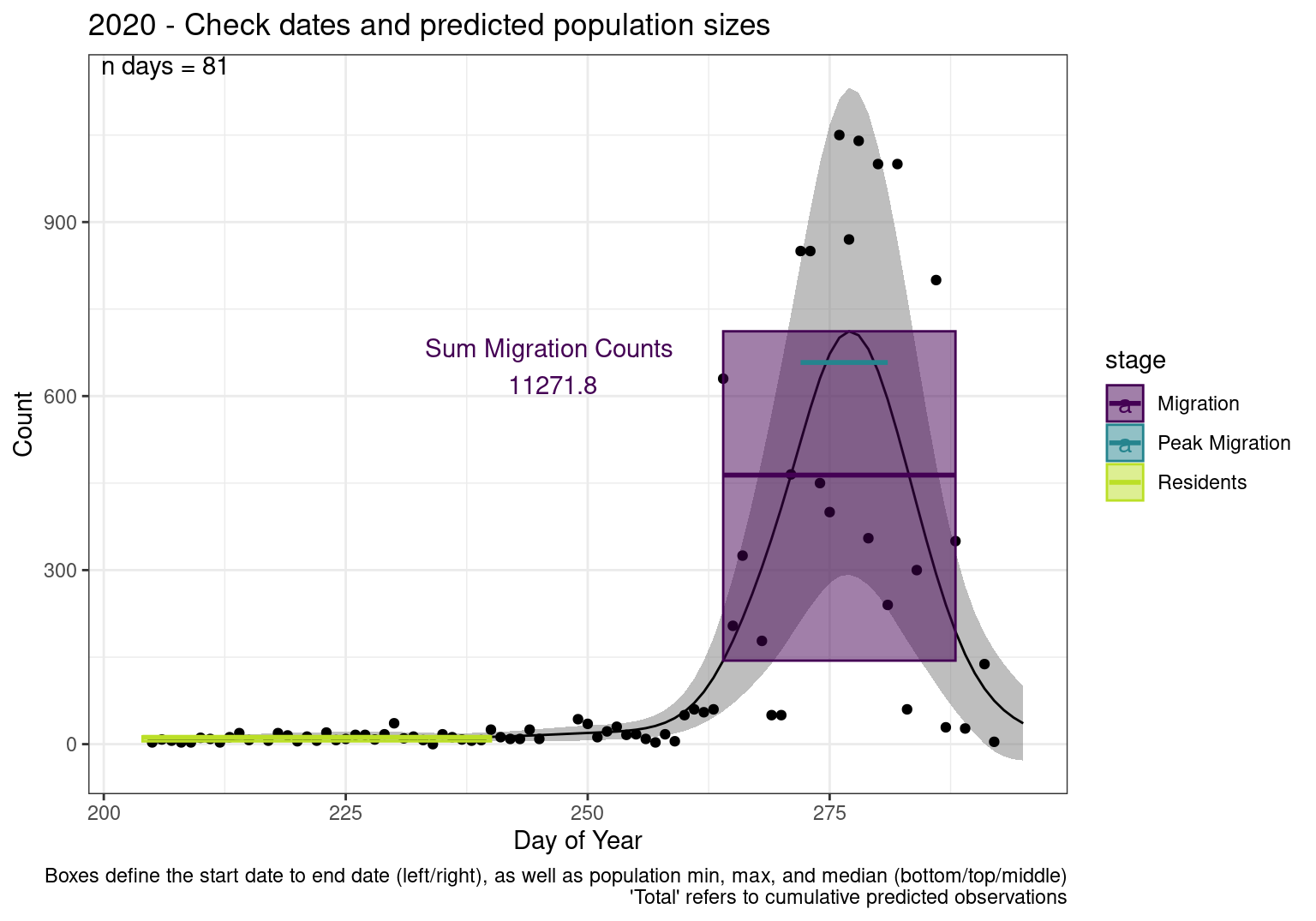
Warning: Removed 1 row containing missing values or values outside the scale range
(`geom_rect()`).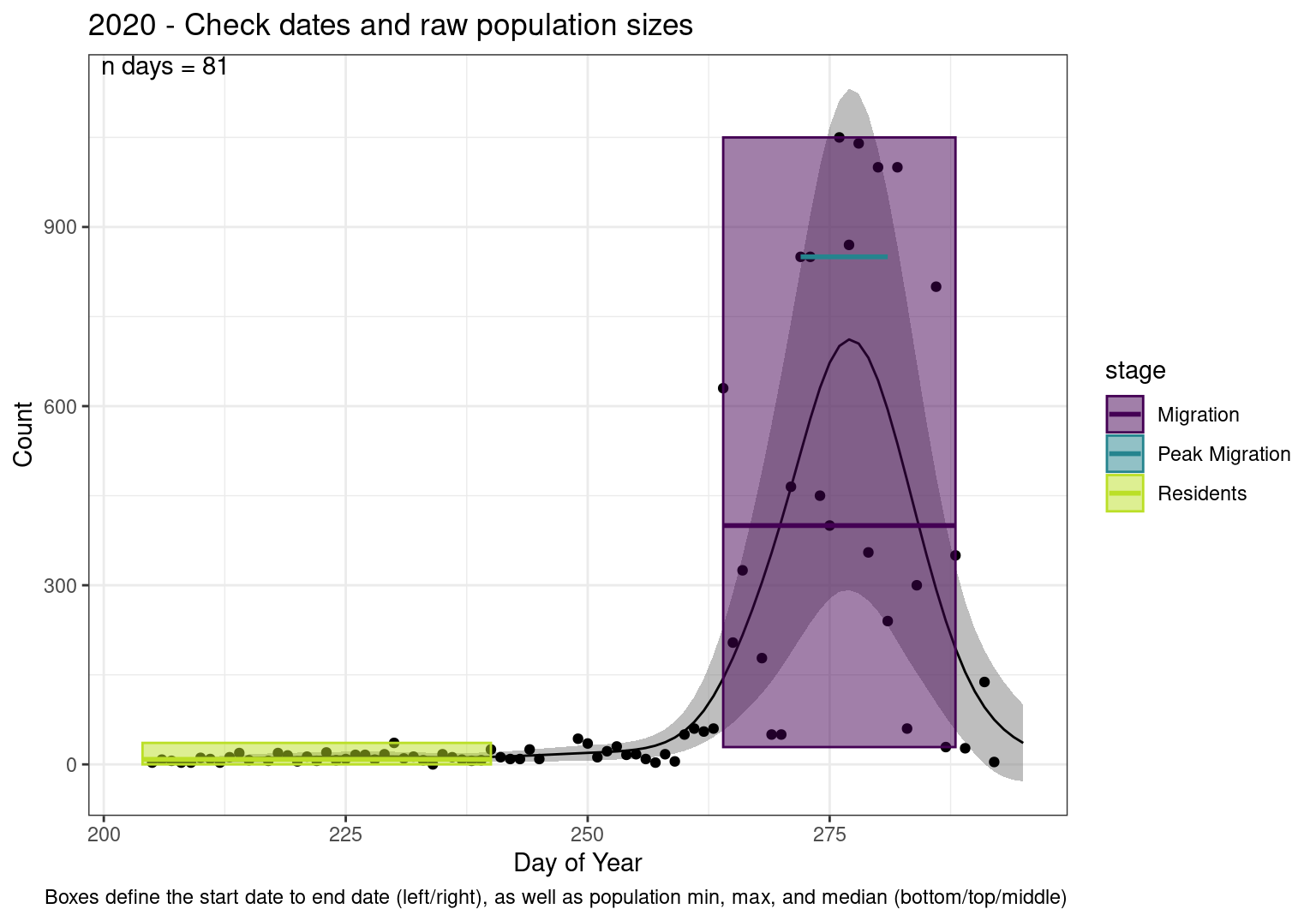
2022
Warning: Removed 1 row containing missing values or values outside the scale range
(`geom_rect()`).
Removed 1 row containing missing values or values outside the scale range
(`geom_text()`).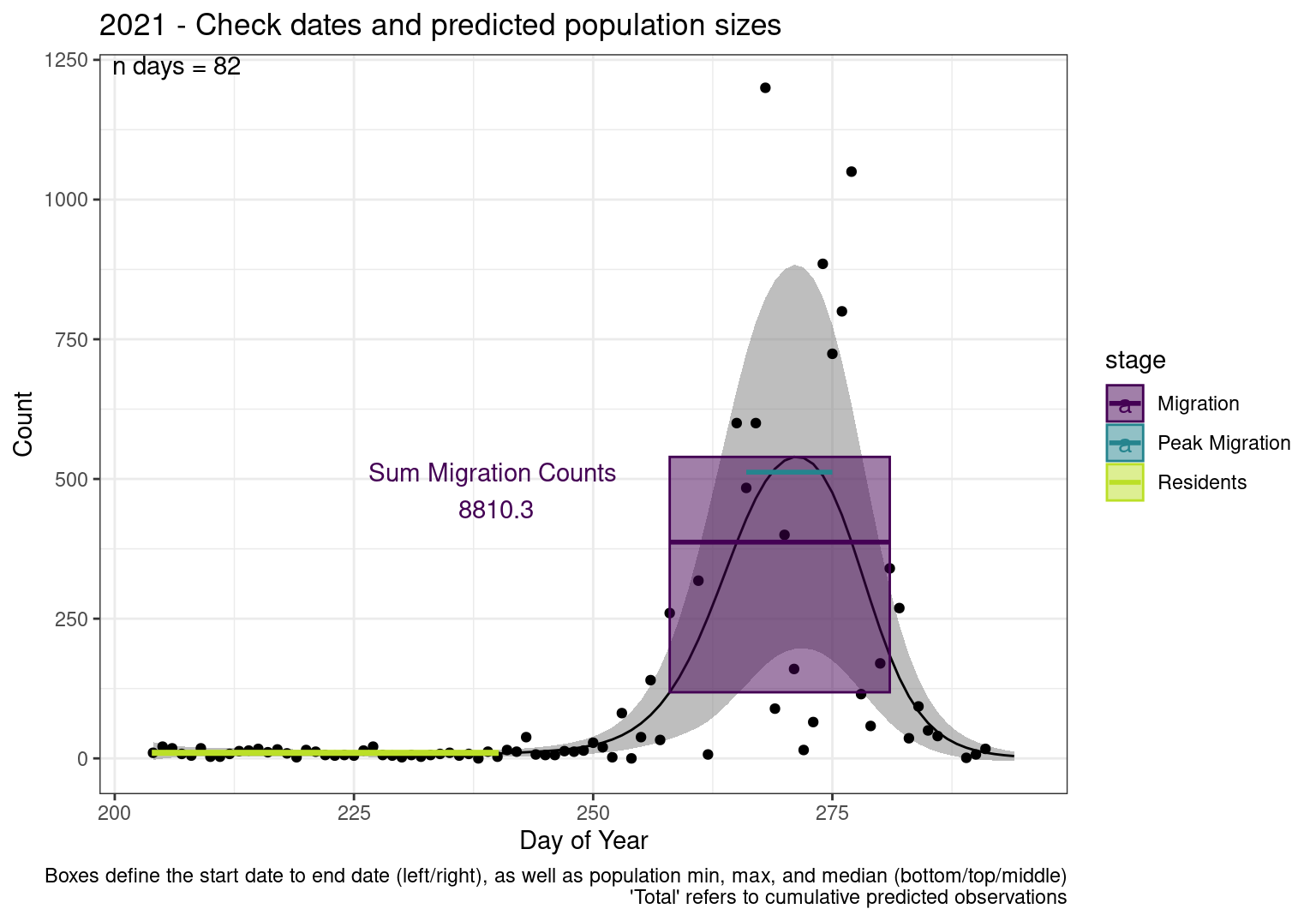
Warning: Removed 1 row containing missing values or values outside the scale range
(`geom_rect()`).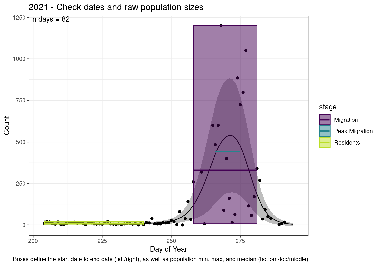
2023
Warning: Removed 1 row containing missing values or values outside the scale range
(`geom_rect()`).
Removed 1 row containing missing values or values outside the scale range
(`geom_text()`).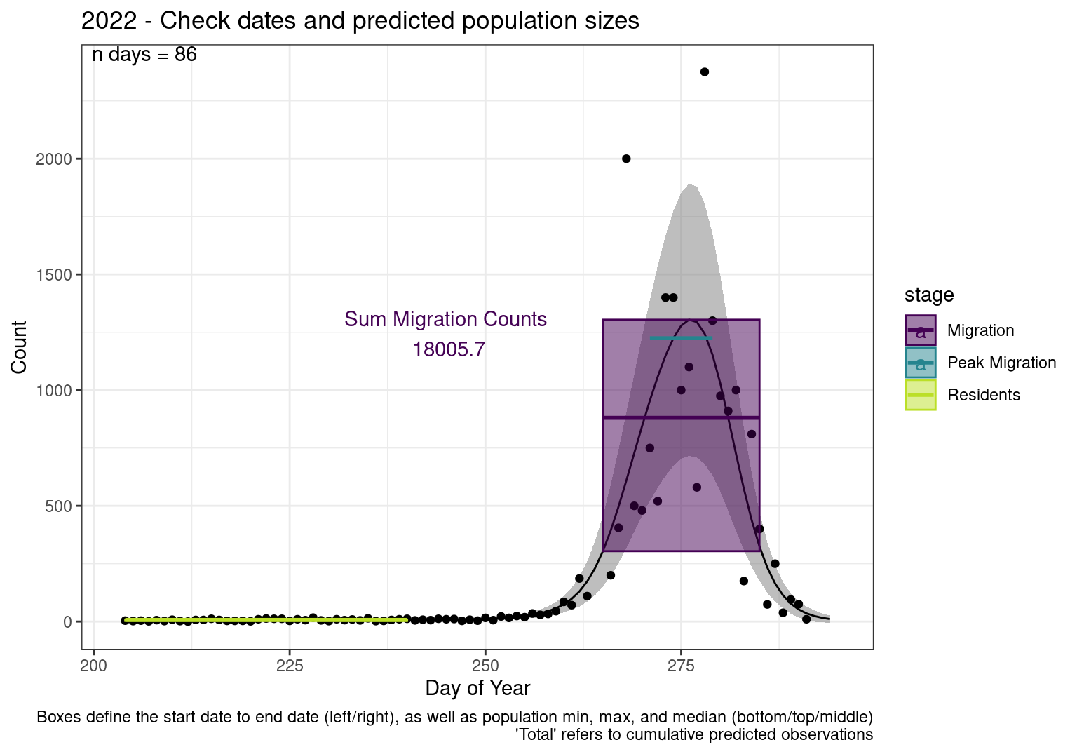
Warning: Removed 1 row containing missing values or values outside the scale range
(`geom_rect()`).