source("XX_setup.R")

recvs <- read_csv("Data/02_Datasets/receivers.csv")
runs <- open_dataset("Data/02_Datasets/runs", format = "feather")Basic Filtering
Here we apply broad filters for missing details, time, space, and species. We’ll omit runs missing deployment information for tags and receivers, runs which occur during times we’re not interested in, and runs which occur for species/receiver pairs which are not within a particular species’ range (ranges were determined in Range Maps), also omitting species we’re not interested in.
The idea is to reduce the size of the data we’re working with as much as possible before we get into the fine details of assessing data quality.
However, we don’t want to simply delete records in our original data because
- we’re working with data which may need to be updated
- if we delete the data we can’t go back if we change our criteria
So we will create lists of all the run/tagID combinations to be removed, and we’ll store these as a new dataset.
When we want to calculate our final summaries, we can apply these filters in the last step before collect()ing (flattening) the feather data files.
Setup
Non-deployments
Both tags and receivers have device ids and deployment ids. Deployments are associated with a particular device (tag or receiver) being deployed at a certain time.
Many erroneous runs are associated with a tag at a time in which that tag was not recorded as deployed.
Funnily enough this can also occur with receivers where the run occurs at a time where the associated receiver is not recorded as deployed.
This could occur for several reasons:
- The metadata is incorrect and the tag/receiver was, in fact deployed at that time
- This is false positive recording of the tag
- This is non-trustworthy receiver data, which may have been collecting during testing or installation
As we cannot be sure which is correct, for now we will omit those runs.
In our custom runs tables, any run/tag combination with missing a tagDeployID or a recvDeployID did not actually have a record of the tag/receiver being deployed at that time.
no_deps <- filter(runs, is.na(speciesID) | is.na(recvDeployID)) |>
  collect()
To be sure that we’re not missing things, we’ll explore what is removed if we use tagDeployID rather than speciesID (as we could conceivably have tags with a deploy id but not species ids).
no_tag_dep_check <- filter(runs, is.na(tagDeployID))For example, in this project for this tag, we have no species ids for a series of runs.
no_tag_dep_check |>
  select(tagID, tagDeployID, speciesID, tsBegin, tsEnd, motusFilter) |>
  filter(tagID == 63138) |>
  collect_ts()
# A tibble: 301 × 6
tagID tagDeployID speciesID tsBegin tsEnd
<int> <int> <int> <dttm> <dttm>
1 63138 NA NA 2022-01-15 10:27:31 2022-01-15 10:28:51
2 63138 NA NA 2022-01-16 04:26:10 2022-01-16 04:26:50
3 63138 NA NA 2022-01-27 01:22:06 2022-01-27 01:22:45
4 63138 NA NA 2022-04-11 20:25:47 2022-04-11 20:27:07
5 63138 NA NA 2022-04-02 21:10:25 2022-04-02 21:11:45
6 63138 NA NA 2022-05-30 21:39:44 2022-05-30 21:41:04
7 63138 NA NA 2022-06-02 22:34:33 2022-06-02 22:35:53
8 63138 NA NA 2022-02-14 19:55:01 2022-02-14 19:55:41
9 63138 NA NA 2022-05-01 01:58:15 2022-05-01 01:59:34
10 63138 NA NA 2022-07-01 10:04:21 2022-07-01 10:05:41
# ℹ 291 more rows
# ℹ 1 more variable: motusFilter <dbl>Note that the motusFilter is also 0, indicating that they are likely false positives based on other metrics as well.
Now if we look at the tag deployment dates for that tag, we see that these runs occurred even before the tag was deployed, further indicating that they are false positives.
runs |>
  filter(tagID == 63138) |>
  select(tagID, tagDeployID,  tsStartTag, tsEndTag, speciesID) |>
  distinct() |>
  collect_ts()
# A tibble: 2 × 5
tagID tagDeployID tsStartTag tsEndTag speciesID
<int> <int> <dttm> <dttm> <int>
1 63138 NA NA NA NA
2 63138 52117 2023-11-10 17:15:00 2025-08-10 17:15:00 19060However, just because we have a tagDeployID, it doesn’t necessarily mean we have a speciesID.
But in all cases where there is a tagDeployID but there is not a speciesID, it’s because the tag is a test tag (test = 1).
runs |>
  filter(!is.na(tagDeployID), is.na(speciesID)) |>
  select(tagID, tagDeployID, test) |>
  distinct() |>
  collect()
# A tibble: 13 × 3
tagID tagDeployID test
<int> <int> <int>
1 52917 32346 1
2 23608 12511 1
3 26315 16538 1
4 26448 13848 1
5 68906 42671 1
6 52918 33943 1
7 64024 38571 1
8 68914 42527 1
9 74330 45876 1
10 74328 45833 1
11 74328 45874 1
12 74331 45877 1
13 74329 45875 1Therefore, we can actually remove all records with missing species ids without worry.
For example, in this project (484) for this receiver device ID (3071), we have no deployment ids (recvDeployID) for a series of runs.
filter(runs, is.na(recvDeployID)) |>
  select(proj_id, recvDeployID, recvDeviceID) |>
  distinct() |>
  collect()
# A tibble: 501 × 3
proj_id recvDeployID recvDeviceID
<int> <int> <int>
1 168 NA 660
2 352 NA 2637
3 352 NA 2635
4 352 NA 1948
5 352 NA 2082
6 352 NA 1855
7 352 NA 1825
8 352 NA 2380
9 352 NA 2173
10 352 NA 2439
# ℹ 491 more rowsfilter(runs, is.na(recvDeployID)) |>
filter(proj_id == 484, recvDeviceID == 3071) |>
select(proj_id, runID, recvDeployID, recvDeviceID, tagDeployID) |>
collect_ts()# A tibble: 40 × 5
proj_id runID recvDeployID recvDeviceID tagDeployID
<int> <int> <int> <int> <int>
1 484 540827863 NA 3071 41246
2 484 540827867 NA 3071 41246
3 484 540827898 NA 3071 41246
4 484 540827900 NA 3071 41246
5 484 540827914 NA 3071 41246
6 484 540827956 NA 3071 41246
7 484 540827975 NA 3071 41243
8 484 540827979 NA 3071 41246
9 484 540827997 NA 3071 41243
10 484 540828021 NA 3071 41246
# ℹ 30 more rowsNow if we look at the receiver deployment dates for that device, we see that these runs occurred before the receiver was deployed, although not that much earlier.
Perhaps these are semi-legitimate runs, which were detected when testing and installing the receiver.
tbl(dbs[["484"]], "recvDeps") |>
  filter(deviceID == "3071") |>
  select(deviceID, deployID, projectID, tsStart, tsEnd, status) |>
  collect_ts()
# A tibble: 1 × 6
deviceID deployID projectID tsStart tsEnd status
<int> <int> <int> <dttm> <dttm> <chr>
1 3071 9150 354 2022-10-18 18:37:00 NA activeTime
In this filter, we omit times of year that don’t apply to our study. This is the easiest filter to apply as it doesn’t rely on metadata or other variables.
Which dates do we keep?
- Fall and Spring migration
- August - December & February - July
Get all runs that are NOT within these dates (Jan, July, Dec)
noise_time <- runs |>
  filter(monthBegin %in% c(1, 7, 12)) |>
  collect()
d <- runs |>
filter(proj_id == 464) |>
mutate(omit = if_else(monthBegin %in% c(1, 7, 12), TRUE, FALSE)) |>
select(runID, tagID, tsBegin, omit, timeBegin) |>
collect()
ggplot(data = d, aes(x = timeBegin, y = factor(tagID), colour = omit)) +
theme_bw() +
geom_point() +
scale_color_viridis_d(end = 0.8)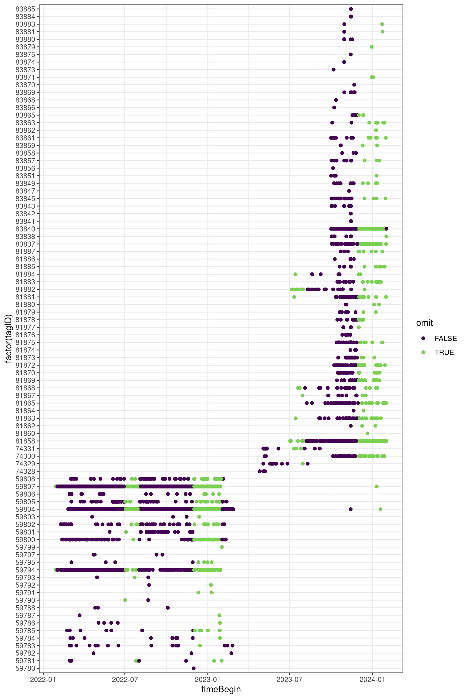
Space
Here we identify runs which are not associated with appropriate stations as determined by overlap with a species range map (Range Maps).
These are runs associated with a species which is unlikely to be found at that station and can therefore be assumed to be false positives.
Note that this step also omits species we’re not interested in, as they are not included in the list of species ranges and receivers.
First we’ll add the master list of whether or not a species is in range for each receiver deployment.
rs <- recvs |>
  mutate(speciesID = as.integer(id),
         recvDeployID = as.integer(recvDeployID)) |>
  filter(in_range) |>
  select(speciesID, recvDeployID, in_range)
Now, get all runs which are NOT in range given the species and the receiver deployment.
noise_space <- runs |>
  left_join(rs, by = c("recvDeployID", "speciesID")) |>
  filter(is.na(in_range)) |>
  select(-"in_range") |>
  collect()
Many of these omitted are omitted because they are missing the speciesID or the recevDeployID (which is already accounted for the the Non-deployments section above.
However, let’s take a look at the remaining ones to check.
Hmm, most of these are poor quality runs (i.e. the motusFilter is 0). So this is a good sign that these are indeed false positives which should be omitted.
noise_space |>
  filter(!is.na(speciesID), !is.na(recvDeployID)) |>
  count(proj_id, motusFilter) |>
  collect() |>
  gt() |>
gt_theme()| proj_id | motusFilter | n |
|---|---|---|
| 168 | 0 | 685 |
| 352 | 0 | 1574 |
| 352 | 1 | 11 |
| 364 | 0 | 1866 |
| 364 | 1 | 275 |
| 373 | 0 | 72 |
| 393 | 0 | 18134 |
| 393 | 1 | 68 |
| 417 | 0 | 10861 |
| 417 | 1 | 8 |
| 464 | 0 | 1536 |
| 464 | 1 | 3 |
| 484 | 0 | 28156 |
| 484 | 1 | 76 |
| 515 | 0 | 389 |
| 515 | 1 | 2 |
| 551 | 0 | 1700 |
| 551 | 1 | 5 |
| 607 | 0 | 95 |
Let’s take a closer look at one species in one project.
There is quite possibly a lot of noise (see the amount of scatter in the motusFilter = 0 category. And clearly this individual (Spotted Towhee) had a home base in southern BC.
ns <- noise_space |>
  filter(proj_id == 484, speciesID == 18550) |>
  select("runID", "tagID") |>
  mutate(in_range = 0)

coords <- tbl(dbs[["484"]], "recvDeps") |>
  select("deployID", "latitude", "longitude") |>
  collect()

rn <- filter(runs, proj_id == 484, speciesID == 18550) |>
  left_join(coords, by = c("recvDeployID" = "deployID")) |>
  left_join(ns, by = c("runID", "tagID")) |>
  filter(!is.na(latitude), !is.na(longitude)) |>
  select(motusFilter, tagDeployID, tsBegin, tsEnd, in_range, latitude, longitude) |>
  collect() |>
  mutate(in_range = factor(replace_na(in_range, 1)))

map <- ne_countries(country = c("Canada", "United States of America"), returnclass = "sf")

rn_sf_cnt <- rn |>
  summarize(n = n(), .by = c("motusFilter", "in_range", "latitude", "longitude")) |>
  st_as_sf(coords = c("longitude", "latitude"), crs = 4326)

ggplot(rn_sf_cnt) +
  geom_sf(data = map) +
  geom_sf(aes(colour = in_range, size = n)) +
  facet_wrap(~motusFilter)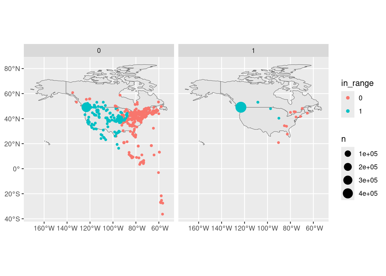
Duplicate runIDs
Double check that there are no duplicate runIDs, which can happen when joining all the data together if we don’t account for duplicate/overlapping receiver/tag deployments.
Additionally there are some duplicates based on the same runID in different batches… This occurs in allruns too, so isn’t an artifact of the custom joins, but still not ideal.
These should have been dealt with in custom_runs() but just in case, we’ll verify here.
runs |>
  count(runID) |>
  filter(n > 1) |>
  collect()
# A tibble: 0 × 2
# ℹ 2 variables: runID <int>, n <int>Okay, good, there are zero duplicates (zero rows).
Looking at the filters
First we’ll combine and collect the ‘bad’ runs.
noise <- bind_rows(no_deps, noise_time, noise_space) |>
  distinct()
Next we’ll take a look at how this compares to the motusFilter.
Original runs
count(runs, proj_id, motusFilter) |>
  filter(proj_id == 484) |>
  collect() |>
  arrange(motusFilter)
# A tibble: 2 × 3
proj_id motusFilter n
<int> <dbl> <int>
1 484 0 492931
2 484 1 601907Remaining (non-bad) runs
anti_join(runs, noise, by = c("runID", "tagDeployID", "recvDeployID")) |>
  filter(proj_id == 484) |>
  count(proj_id, motusFilter) |>
  collect()
# A tibble: 2 × 3
proj_id motusFilter n
<int> <dbl> <int>
1 484 0 336867
2 484 1 429134There are still many remaining ‘bad’ data (according to the motusFilter)… perhaps we should use that as well, or see what happens after we do the next stage of fine scale filtering.
Saving filters
We’ll save the ‘bad data’ for use in the next steps.
write_feather(noise, sink = "Data/02_Datasets/noise_runs.feather")Wrap up
Disconnect from the databases
walk(dbs, dbDisconnect)