source("XX_setup.R")
runs <- load_runs()
meta <- runs |>
  select(tagDeployID, speciesID) |>
  distinct() |>
  left_join(tbl(dbs[[1]], "species") |> select(english, id) |> collect(),
            by = c("speciesID" = "id"))

bouts <- read_rds("Data/02_Datasets/bouts_cleaned.rds") |>
  left_join(meta, by = "tagDeployID")
trans <- read_rds("Data/02_Datasets/transitions_cleaned.rds") |>
left_join(meta, by = "tagDeployID")Summaries
In this script we will finalize the data sets by adding metadata and summarizing as appropriate. Each data set will be saved to CSV file for future analysis (see Appendix - Data for descriptions of the data values).
Setup
Adding metadata
Add appropriate meta data for summaries as well as for creating final datasets. Ensure datasets now include all the meta data and have been converted to flat files (no list columns, no specially column formats, such as durations or difftimes), so can now be saved to csv.
Datasets created:
trans <- trans |>
  # Omit weird metrics
  select(-"migration", -"connected") |>
  # Flatten units
  mutate(min_time_hrs = flatten_units(min_time, "hours"),
         time_diff_hrs = flatten_units(time_diff, "hours"),
         next_dist_km = flatten_units(next_dist, "km"),
         lag1_min = flatten_units(lag1, "min"),
         lag2_min = flatten_units(lag2, "min"),
         speed_m_s = flatten_units(speed, "m/s"))|>
  select(-min_time, -time_diff, -lag1, -lag2, -speed)

tz <- bouts |>
  select(dateBegin, recvDeployLat, recvDeployLon) |>
  distinct() |>
  mutate(tz = tz_lookup_coords(recvDeployLat, recvDeployLon, warn = FALSE),
         offset = map2(dateBegin, tz, tz_offset)) |>
  unnest(offset) |>
  select("dateBegin", "recvDeployLat", "recvDeployLon", "utc_offset_h")

bouts <- left_join(bouts, tz, by = c("dateBegin", "recvDeployLat", "recvDeployLon")) |>
  # Add local times
  mutate(timeBeginLocal = timeBegin + hours(utc_offset_h),
         timeEndLocal = timeEnd + hours(utc_offset_h)) |>
  select(-"runID", -"len", -"ant") |>  # Omit list columns
  # Flatten units
  mutate(total_time = flatten_units(total_time, "min")) |>
  rename(total_time_min = total_time)

write_csv(bouts, "Data/03_Final/bouts_final.csv")
write_csv(trans, "Data/03_Final/transitions_final.csv")
Daily summaries
Summarize how much time each individual spent at a particular station on a given day.
Here we will work in local times to determine when a day rolls over at midnight. We will then split each bout that crosses midnight into multiple bouts, each starting and stopping at the day’s limits (midnight).
Then we’ll summarize these data into amount of time spent per day at a spectific station.
Datasets created:
plan(multisession, workers = 6) # Setup parallel

bouts_split <- bouts |>
  mutate(
    # Split bouts by days
    date_local = future_map2(timeBeginLocal, timeEndLocal, \(x, y) {
      if(as_date(x) != as_date(y)) {
        d <- seq(as_date(x), as_date(y), by = "1 day")
        d <- d[d >= x & d <= y]
      } else d <- c()
      unique(c(x, d, y))
    }, .progress = interactive()),
    t1 = map(date_local, \(x) x[-length(x)]),
    t2 = map(date_local, \(x) x[-1]),
  ) |>
  unnest(cols = c(t1, t2)) |>
  select(-dateBegin, -timeBegin, -timeEnd, -timeBeginLocal, -timeEndLocal, -date_local) |>
  rename(timeBeginLocal = t1, timeEndLocal = t2) |>
  mutate(dateBeginLocal = as_date(timeBeginLocal))

daily_bouts <- bouts_split |>
  summarize(time_hrs = sum(difftime(timeEndLocal, timeBeginLocal, units = "hours")),
            time_hrs = as.numeric(time_hrs),
            .by = c("english", "tagDeployID", "stn_group", "dateBeginLocal")) |>
  # Add in lat/lon (corresponds to one of the stations, not all in a group, but close enough)
  left_join(select(bouts, "stn_group", "recvDeployLat", "recvDeployLon") |> distinct(),
            by = "stn_group")

write_csv(daily_bouts, "Data/03_Final/bouts_final_split.csv")
write_csv(daily_bouts, "Data/03_Final/summary_daily_bouts.csv")
Individual Summaries
Summarize the individual and overall patterns and number of samples in the data.
We’ll categorize birds as those who we know
- Did not travel
travelled(moved at least 100 km)migrated(moved at least 1 latitude ~111km south/north)migrated_far(moved at least 5 latitudes ~555km south/north)- Overall (across all birds)
This doesn’t mean that birds didn’t move farther, only that we have no evidence that they did.
Datasets created:
trans_dist <- trans |>
  summarize(total_dist = sum(next_dist),
            travelled = total_dist > set_units(100, "km"),
            migrated = (max(lat1) - min(lat2)) > 1,
            migrated_far = (max(lat1) - min(lat2)) > 5,
            .by = c("english", "tagDeployID"))

sum_time <- daily_bouts |>
  left_join(trans_dist, by = c("english", "tagDeployID")) |>
  mutate(total_dist = replace_na(total_dist, set_units(0, "km")),
         travelled = replace_na(travelled, FALSE),
         migrated = replace_na(migrated, FALSE),
         migrated_far = replace_na(migrated_far, FALSE)) |>
  arrange(tagDeployID, dateBeginLocal) |>
  summarize(n_stn = n_distinct(stn_group),
            min_date = min(dateBeginLocal),
            mean_date = mean(dateBeginLocal),
            max_date = max(dateBeginLocal),
            total_time_hrs = sum(time_hrs),
            mean_time_hrs = mean(time_hrs),
            res_stn = stn_group[1],
            mean_time_no_resident_hrs = mean(time_hrs[stn_group != stn_group[1]]),
            first_time_hrs = sum(time_hrs[stn_group == stn_group[1]]),
            last_time_hrs = sum(time_hrs[stn_group == stn_group[n()]]),
            .by = c("english", "tagDeployID", "travelled", "migrated", "migrated_far")
  ) |>
  mutate(mean_time_no_resident_hrs = replace_na(mean_time_no_resident_hrs, 0)) |>
  mutate(across(where(is.difftime), as.numeric))

write_csv(sum_time, "Data/03_Final/summary_birds.csv")
Now we’ll create an overall summary of these individual-level summaries. This is a summary table looking at the sample sizes (No. XXX) as well as averages of individual means (Avg of mean etc.).
Code
sum_time |>
  bind_rows(mutate(sum_time, travelled = FALSE, migrated = FALSE,
                   migrated_far = FALSE, overall = TRUE)) |>
  summarize(n = n(),
            n_species = n_distinct(english),
            across(-c("tagDeployID", "res_stn", "english", "min_date", "max_date"), mean),
            min_date = min(min_date), max_date = max(max_date),
            .by = c("travelled", "migrated", "migrated_far", "overall")) |>
  mutate(type = case_when(overall ~ "Overall",
                          migrated_far ~ "Migrated Far (>5 Latitudes)",
                          migrated ~ "Migrated (>1 Latitude)",
                          travelled ~ "Travelled (>100km)",
                          TRUE ~ "No large movements")) |>
  select(-travelled, -migrated, -migrated_far, -overall) |>
  select(`No. Individuals` = "n",
         `No. Species` = "n_species",
         `Avg. No. Stations visited` = "n_stn",
         `Min date` = "min_date",
         `Avg date` = "mean_date",
         `Max date` = "max_date",
         `Avg total time detected` = "total_time_hrs",
         `Avg mean time detected` = "mean_time_hrs",
         `Avg mean time detected (not at resident station)` = "mean_time_no_resident_hrs",
         `Avg total time detected by resident station` = "first_time_hrs",
         `Avg total time detected by final station` = "last_time_hrs",
         type) |>
  mutate(across(where(is.numeric), \(x) round(x, 2))) |>
  pivot_longer(-type, names_to = "Measure", values_transform = as.character) |>
  pivot_wider(names_from = "type") |>
  select("Measure", contains("No large"), contains("Trave"), contains(">1"), contains(">5"), "Overall") |>
  gt() |>
  gt_theme() |>
tab_header(title = "Overall summary")| Overall summary | |||||
|---|---|---|---|---|---|
| Measure | No large movements | Travelled (>100km) | Migrated (>1 Latitude) | Migrated Far (>5 Latitudes) | Overall |
| No. Individuals | 535 | 30 | 167 | 330 | 1062 |
| No. Species | 36 | 12 | 18 | 21 | 39 |
| Avg. No. Stations visited | 1.02 | 2.53 | 3.17 | 4.61 | 2.52 |
| Min date | 2014-11-07 | 2018-08-05 | 2014-10-09 | 2017-07-31 | 2014-10-09 |
| Avg date | 2022-01-18 | 2022-08-01 | 2022-02-17 | 2022-02-28 | 2022-02-10 |
| Max date | 2023-12-01 | 2023-11-26 | 2023-11-26 | 2023-11-25 | 2023-12-01 |
| Avg total time detected | 390.86 | 300.1 | 352.12 | 290.53 | 351.03 |
| Avg mean time detected | 8.16 | 5.78 | 9.21 | 9.29 | 8.61 |
| Avg mean time detected (not at resident station) | 0.01 | 0.29 | 0.27 | 0.27 | 0.14 |
| Avg total time detected by resident station | 390.83 | 298.86 | 351.14 | 288.11 | 350.07 |
| Avg total time detected by final station | 386.83 | 24.48 | 1.65 | 19.71 | 201.95 |
Looking for stopovers
Are there any individuals that actually hang out around the receiver?
We’ll look for two different indicators of a stopover
- Actually being detected around a receiver for longer than half an hour
- In the above summaries, we see that the average amount of time detected at a receiver which is not the first (or home) receiver, is about 9min (0.15 hours)
- Being detected around a single receiver (or receiver group) on more than one day each detection within a week of another (and no other stations detected in the meanwhile).
So looking only at October through April (months 10-4), we’ll define some stopover metrics.
Datasets created:
stopovers <- daily_bouts |>
  arrange(tagDeployID, dateBeginLocal) |>
  filter(stn_group != stn_group[1],
         month(dateBeginLocal) %in% c(10, 11, 12, 1, 2, 3, 4), .by = "tagDeployID") |>
  mutate(
    # Detected at the same station across days?
    same_stn = stn_group == lead(stn_group, default = "x"),
    same_stn = same_stn | lag(same_stn, default = FALSE),
    # Detected within 7 days?
    close_time = dateBeginLocal >= (lead(dateBeginLocal, default = ymd("2999-01-01")) - days(7)),
    close_time = close_time | lag(close_time, default = FALSE),
    # If both, call this a multi-day stopover
    stopover = same_stn & close_time,
    .by = "tagDeployID")
Over 30 min at a receiver
Here we see different individuals spending time around receivers during migration.
stopover_time <- stopovers |>
  group_by(english, tagDeployID) |>
  select(-same_stn, -close_time, -stopover) |>
  arrange(english, tagDeployID) |>
  filter(time_hrs > 0.5)
write_csv(stopover_time, "Data/03_Final/summary_stopover_time.csv")

stopover_time |>
  select(-"recvDeployLat", -"recvDeployLon") |>
  gt() |>
  gt_theme() |>
  fmt_number(columns = time_hrs) |>
  cols_label_with(everything(), tools::toTitleCase) |>
  cols_label(time_hrs ~ "Time ({{Hours}})") |>
  tab_options(container.height = px(600),
              container.overflow.y = "auto") |>
tab_caption("Stopovers >30min (see Time (Hours) column)")| Stn_group | dateBeginLocal | Time (Hours) |
|---|---|---|
| Blue-headed Vireo - 50721 | ||
| 8934 | 2023-10-18 | 0.51 |
| Blue-headed Vireo - 50722 | ||
| 8056-8374 | 2023-10-19 | 0.72 |
| Blue-headed Vireo - 51153 | ||
| 7429-8056 | 2023-11-05 | 0.51 |
| Chestnut-collared Longspur - 40626 | ||
| 8603 | 2022-10-30 | 0.65 |
| Golden-crowned Sparrow - 44345 | ||
| 5216-8159-8296-8415-9233 | 2023-10-05 | 0.93 |
| Golden-crowned Sparrow - 44358 | ||
| 8180 | 2023-04-29 | 0.86 |
| Gray Catbird - 26019 | ||
| 3817-4379-5820 | 2019-10-09 | 0.54 |
| Gray Catbird - 29769 | ||
| 5885-5886 | 2020-10-12 | 0.57 |
| Hermit Thrush - 43517 | ||
| 4205-5146-6065-7400 | 2022-10-28 | 0.71 |
| Hermit Thrush - 43669 | ||
| 5439-5838 | 2022-10-29 | 0.73 |
| Hermit Thrush - 50944 | ||
| 9120-10290 | 2023-10-25 | 10.68 |
| 9120-10290 | 2023-10-26 | 2.96 |
| Hermit Thrush - 51150 | ||
| 8858 | 2023-11-06 | 10.13 |
| Pine Siskin - 2661 | ||
| 1111 | 2014-10-24 | 0.52 |
| Purple Finch - 38289 | ||
| 7419 | 2022-10-03 | 0.53 |
| Purple Finch - 38290 | ||
| 5146-6065-7400 | 2023-04-23 | 1.74 |
| Purple Finch - 38291 | ||
| 8934 | 2022-10-29 | 7.12 |
| 8934 | 2022-10-30 | 7.37 |
| Purple Finch - 38296 | ||
| 7416-7419-8148-9207 | 2022-10-03 | 0.88 |
| Purple Finch - 38303 | ||
| 7290-7429 | 2022-11-19 | 0.51 |
| Purple Finch - 38944 | ||
| 6065-7400 | 2022-10-28 | 5.11 |
| 6065-7400 | 2022-10-29 | 0.58 |
| Purple Finch - 45363 | ||
| 7763 | 2023-11-17 | 11.31 |
| 7763 | 2023-11-18 | 7.85 |
| Song Sparrow - 34483 | ||
| 4748 | 2021-10-13 | 0.81 |
| Song Sparrow - 39553 | ||
| 2429-7756-8251-9097 | 2022-10-23 | 0.74 |
| Song Sparrow - 39581 | ||
| 9114 | 2022-10-24 | 0.66 |
| 7218-7756-8100-8946-9097-9123 | 2022-10-24 | 0.67 |
| Song Sparrow - 42558 | ||
| 7469-7932 | 2022-10-28 | 0.57 |
| Song Sparrow - 43000 | ||
| 8193-8540 | 2022-11-08 | 0.70 |
| Song Sparrow - 43250 | ||
| 2812-7446 | 2022-10-15 | 0.94 |
| 7338 | 2022-10-24 | 0.57 |
| Spotted Towhee - 41242 | ||
| 9032 | 2023-04-12 | 0.68 |
| Sprague's Pipit - 40850 | ||
| 7450-7484-7510-7511 | 2022-10-27 | 0.74 |
| Swainson's Thrush - 17672 | ||
| 3075-3560 | 2018-10-10 | 0.59 |
| Swainson's Thrush - 18903 | ||
| 4971 | 2018-10-12 | 0.63 |
| Swainson's Thrush - 19414 | ||
| 4705 | 2018-10-30 | 0.50 |
| Swainson's Thrush - 35486 | ||
| 4599-7633 | 2021-10-08 | 0.53 |
| Swainson's Thrush - 35733 | ||
| 7664-8085 | 2021-10-12 | 0.73 |
| Swainson's Thrush - 35739 | ||
| 5439-5838 | 2021-10-14 | 0.55 |
| Swainson's Thrush - 36312 | ||
| 6127-7261 | 2021-10-04 | 0.56 |
| Swainson's Thrush - 36315 | ||
| 5146-6065-7400-7754 | 2021-10-01 | 0.62 |
| Swainson's Thrush - 41657 | ||
| 6126-6127 | 2022-10-01 | 0.60 |
| Swainson's Thrush - 41675 | ||
| 6127-7261 | 2022-10-05 | 1.39 |
| Swainson's Thrush - 42002 | ||
| 7638-7639 | 2022-10-04 | 0.66 |
| Swainson's Thrush - 42242 | ||
| 6126-6127 | 2022-10-02 | 0.61 |
| Swainson's Thrush - 42244 | ||
| 6125 | 2022-10-11 | 0.70 |
| Swainson's Thrush - 42474 | ||
| 8279 | 2022-11-21 | 0.56 |
| Swainson's Thrush - 42476 | ||
| 4665 | 2022-10-04 | 1.05 |
| Swainson's Thrush - 43016 | ||
| 9465 | 2023-04-30 | 0.68 |
| Swainson's Thrush - 43426 | ||
| 4205-5146-6065-7400 | 2022-10-11 | 0.68 |
| Swainson's Thrush - 44111 | ||
| 9446-9465-10188 | 2023-10-13 | 1.01 |
| Swainson's Thrush - 49419 | ||
| 8835 | 2023-10-04 | 0.57 |
| Western Meadowlark - 40712 | ||
| 8681 | 2023-03-17 | 0.72 |
| Western Meadowlark - 47322 | ||
| 8316 | 2023-10-22 | 0.56 |
| 10308 | 2023-10-23 | 0.53 |
| Western Meadowlark - 47334 | ||
| 8345-10443 | 2023-10-15 | 0.91 |
| White-throated Sparrow - 34474 | ||
| 5398-7354 | 2021-10-19 | 10.10 |
| 5398-7354 | 2021-10-20 | 13.10 |
| 5398-7354 | 2021-10-21 | 14.31 |
| 5398-7354 | 2021-10-22 | 1.19 |
| 5398-7354 | 2021-10-23 | 1.47 |
| 5398-7354 | 2021-10-24 | 3.71 |
| 5398-7354 | 2021-10-25 | 5.99 |
| 5398-7354 | 2021-10-26 | 6.54 |
| 5398-7354 | 2021-10-27 | 0.73 |
| Yellow-rumped Warbler (Myrtle) - 43346 | ||
| 6208-7432-8661 | 2022-10-18 | 0.52 |
Examples
plot_map(trans, 43250) +
  labs(title = "Song Sparrow",
       caption = "Spent 1 hour at 2812-7446 on October 15th and 30min at 7338 on Oct 24th")
Loading required namespace: rasterZoom: 7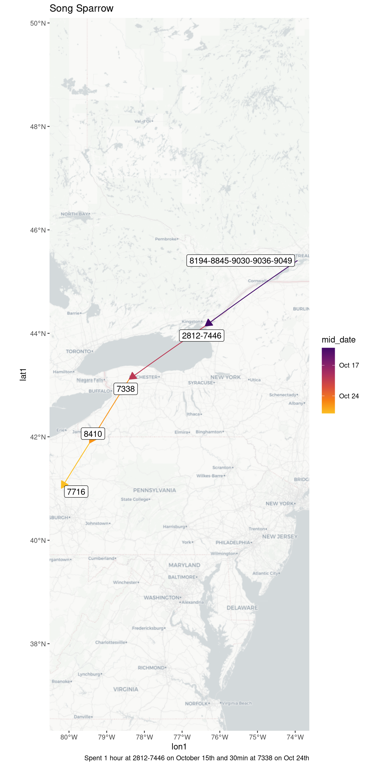
plot_map(trans, 51150) +
  labs(title = "Hermit Thrush",
       caption = "Spent 10 hours at 8858 on November 6th")
Zoom: 7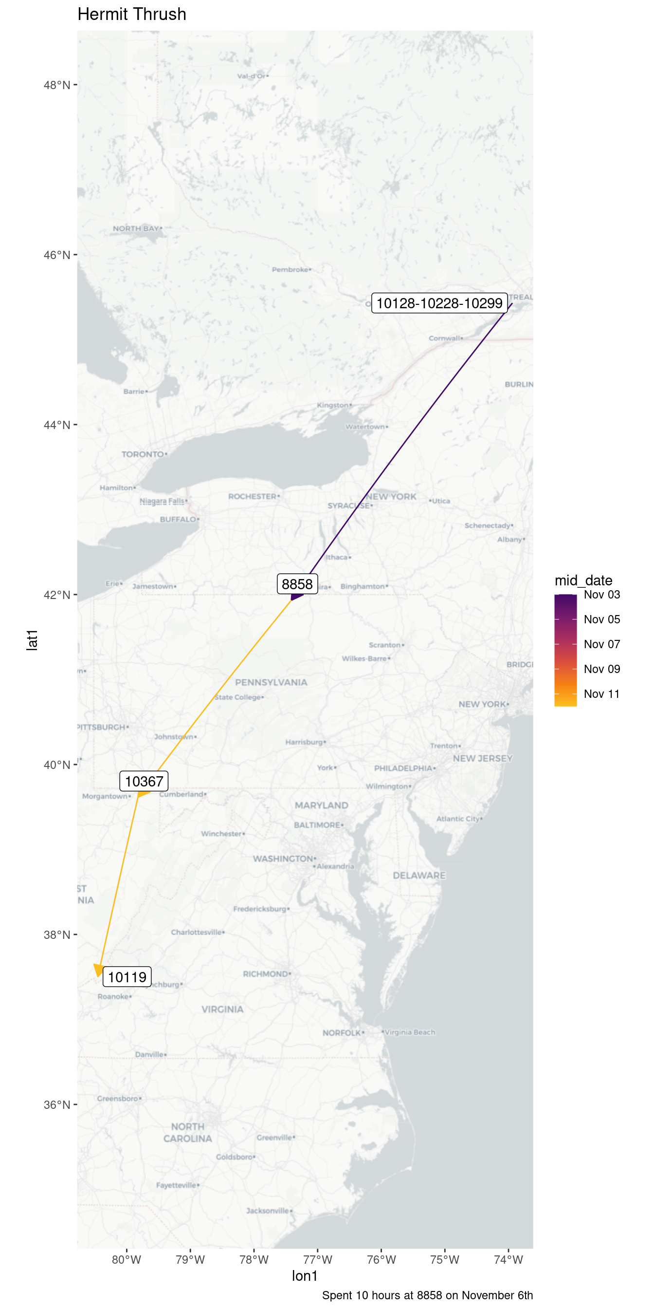
Several days at a receiver
What about individuals which are spotted several days in a row at a station, even if not for a long period of time?
stopover_days <- stopovers |>
  group_by(english, tagDeployID) |>
  filter(stopover) |>
  select(-same_stn, -close_time, -stopover)
write_csv(stopover_days, "Data/03_Final/summary_stopover_days.csv")

stopover_days |>
  select(-"recvDeployLat", -"recvDeployLon") |>
  gt() |>
  gt_theme() |>
  fmt_number(columns = time_hrs) |>
  cols_label_with(everything(), tools::toTitleCase) |>
  cols_label(time_hrs ~ "Time ({{Hours}})") |>
  tab_options(container.height = px(600),
              container.overflow.y = "auto") |>
tab_caption("Stopovers where detected over several days at a receiver")| Stn_group | dateBeginLocal | Time (Hours) |
|---|---|---|
| Pine Siskin - 2661 | ||
| 1111 | 2014-10-24 | 0.52 |
| 1111 | 2014-10-25 | 0.28 |
| Swainson's Thrush - 18901 | ||
| 3495-4725-5240 | 2018-10-08 | 0.17 |
| 3495-4725-5240 | 2018-10-09 | 0.13 |
| 3495-4725-5240 | 2018-10-10 | 0.03 |
| Swainson's Thrush - 18902 | ||
| 4665 | 2018-10-07 | 0.35 |
| 4665 | 2018-10-09 | 0.08 |
| Swainson's Thrush - 19412 | ||
| 4665 | 2018-10-11 | 0.04 |
| 4665 | 2018-10-12 | 0.01 |
| Gray Catbird - 29572 | ||
| 3551-4451 | 2020-10-05 | 0.20 |
| 3551-4451 | 2020-10-06 | 0.13 |
| White-throated Sparrow - 34474 | ||
| 5398-7354 | 2021-10-19 | 10.10 |
| 5398-7354 | 2021-10-20 | 13.10 |
| 5398-7354 | 2021-10-21 | 14.31 |
| 5398-7354 | 2021-10-22 | 1.19 |
| 5398-7354 | 2021-10-23 | 1.47 |
| 5398-7354 | 2021-10-24 | 3.71 |
| 5398-7354 | 2021-10-25 | 5.99 |
| 5398-7354 | 2021-10-26 | 6.54 |
| 5398-7354 | 2021-10-27 | 0.73 |
| Song Sparrow - 34492 | ||
| 3787-7756 | 2021-11-03 | 0.15 |
| 3787-7756 | 2021-11-04 | 0.05 |
| Swainson's Thrush - 35740 | ||
| 7240-7261 | 2021-10-06 | 0.23 |
| 7240-7261 | 2021-10-07 | 0.31 |
| Swainson's Thrush - 36312 | ||
| 6127-7261 | 2021-10-04 | 0.56 |
| 6127-7261 | 2021-10-06 | 0.38 |
| Purple Finch - 38291 | ||
| 8934 | 2022-10-29 | 7.12 |
| 8934 | 2022-10-30 | 7.37 |
| Purple Finch - 38303 | ||
| 7290-7429 | 2022-11-18 | 0.17 |
| 7290-7429 | 2022-11-19 | 0.51 |
| 7290-7429 | 2022-11-20 | 0.05 |
| Purple Finch - 38944 | ||
| 6065-7400 | 2022-10-28 | 5.11 |
| 6065-7400 | 2022-10-29 | 0.58 |
| Red-eyed Vireo - 39559 | ||
| 8845 | 2022-10-02 | 0.02 |
| 8845 | 2022-10-03 | 0.01 |
| Song Sparrow - 39561 | ||
| 9193-9194 | 2022-11-19 | 0.02 |
| 9193-9194 | 2022-11-20 | 0.01 |
| Song Sparrow - 39578 | ||
| 7675 | 2022-10-17 | 0.08 |
| 7675 | 2022-10-18 | 0.04 |
| 7735-8306 | 2022-10-18 | 0.03 |
| 7735-8306 | 2022-10-24 | 0.08 |
| Song Sparrow - 39586 | ||
| 3994-8121 | 2022-10-17 | 0.16 |
| 3994-8121 | 2022-10-23 | 0.04 |
| Ovenbird - 39587 | ||
| 9194 | 2022-11-13 | 0.08 |
| 9194 | 2022-11-14 | 0.03 |
| 9194 | 2022-11-19 | 0.08 |
| 9194 | 2022-11-22 | 0.01 |
| Red-eyed Vireo - 39589 | ||
| 9150-9191-9193 | 2022-11-23 | 0.22 |
| 9150-9191-9193 | 2022-11-27 | 0.07 |
| Song Sparrow - 39594 | ||
| 9191-9193-9194 | 2022-10-28 | 0.03 |
| Song Sparrow - 39610 | ||
| 4462-8885 | 2022-11-01 | 0.01 |
| 4462-8885 | 2022-11-02 | 0.27 |
| 9150-9191-9192-9193-9194 | 2022-11-23 | 0.02 |
| 9150-9191-9192-9193-9194 | 2022-11-25 | 0.16 |
| 9150-9191-9192-9193-9194 | 2022-11-30 | 0.11 |
| Song Sparrow - 39611 | ||
| 9193-9194 | 2022-11-24 | 0.05 |
| 9193-9194 | 2022-11-25 | 0.03 |
| Western Meadowlark - 40712 | ||
| 8681 | 2023-03-16 | 0.41 |
| 8681 | 2023-03-17 | 0.72 |
| Swainson's Thrush - 41683 | ||
| 7878 | 2022-10-02 | 0.20 |
| 7878 | 2022-10-03 | 0.01 |
| Swainson's Thrush - 42002 | ||
| 7638-7639 | 2022-10-03 | 0.05 |
| 7638-7639 | 2022-10-04 | 0.66 |
| Swainson's Thrush - 42241 | ||
| 8331-8332 | 2022-10-16 | 0.03 |
| 8331-8332 | 2022-10-21 | 0.11 |
| Swainson's Thrush - 42474 | ||
| 8950 | 2023-03-30 | 0.15 |
| 8950 | 2023-04-05 | 0.06 |
| Swainson's Thrush - 42787 | ||
| 5056-7236 | 2022-10-14 | 0.06 |
| 5056-7236 | 2022-10-15 | 0.08 |
| Swainson's Thrush - 42972 | ||
| 8950 | 2023-04-20 | 0.11 |
| Song Sparrow - 42999 | ||
| 7616 | 2022-10-17 | 0.02 |
| 7616 | 2022-10-18 | 0.36 |
| Swainson's Thrush - 43066 | ||
| 7424-7506 | 2022-10-08 | 0.13 |
| 7424-7506 | 2022-10-10 | 0.30 |
| Swainson's Thrush - 43067 | ||
| 8455 | 2022-10-26 | 0.12 |
| 8455 | 2022-10-27 | 0.02 |
| Song Sparrow - 43250 | ||
| 2812-7446 | 2022-10-15 | 0.94 |
| 2812-7446 | 2022-10-16 | 0.15 |
| Hermit Thrush - 43516 | ||
| 6013-7228 | 2022-10-29 | 0.24 |
| 6013-7228 | 2022-10-30 | 0.06 |
| Northern Cardinal - 43720 | ||
| 5068 | 2023-03-27 | 0.02 |
| 5068 | 2023-03-29 | 0.01 |
| Northern Cardinal - 43779 | ||
| 5068 | 2023-02-27 | 0.12 |
| 5068 | 2023-03-01 | 0.04 |
| 5068 | 2023-03-17 | 0.07 |
| 5068 | 2023-03-24 | 0.13 |
| Northern Cardinal - 43978 | ||
| 5068 | 2023-03-05 | 0.04 |
| 5068 | 2023-03-06 | 0.04 |
| 5068 | 2023-03-07 | 0.11 |
| 5068 | 2023-03-08 | 0.01 |
| 5068 | 2023-03-21 | 0.11 |
| 5068 | 2023-03-23 | 0.04 |
| 5068 | 2023-03-29 | 0.03 |
| Swainson's Thrush - 45239 | ||
| 7429-9697 | 2023-10-11 | 0.15 |
| 7429-9697 | 2023-10-16 | 0.04 |
| Purple Finch - 45363 | ||
| 7763 | 2023-11-17 | 11.31 |
| 7763 | 2023-11-18 | 7.85 |
| Western Meadowlark - 47328 | ||
| 9073-9505 | 2023-10-08 | 0.18 |
| 9073-9505 | 2023-10-12 | 0.32 |
| Swainson's Thrush - 49419 | ||
| 5068-7441 | 2023-10-04 | 0.03 |
| 5068-7441 | 2023-10-07 | 0.16 |
| Yellow-rumped Warbler (Myrtle) - 50428 | ||
| 7424-7469 | 2023-10-12 | 0.11 |
| 7424-7469 | 2023-10-13 | 0.03 |
| 6208-7432-7539-8661 | 2023-10-23 | 0.36 |
| 6208-7432-7539-8661 | 2023-10-24 | 0.10 |
| 6208-7432-7539-8661 | 2023-10-28 | 0.03 |
| Hermit Thrush - 50719 | ||
| 7987-8875 | 2023-10-14 | 0.01 |
| 7987-8875 | 2023-10-16 | 0.03 |
| Yellow-rumped Warbler (Myrtle) - 50939 | ||
| 6124 | 2023-10-23 | 0.13 |
| 6124 | 2023-10-24 | 0.01 |
| Hermit Thrush - 50944 | ||
| 9120-10290 | 2023-10-25 | 10.68 |
| 9120-10290 | 2023-10-26 | 2.96 |
| Swainson's Thrush - 51086 | ||
| 9627 | 2023-11-25 | 0.02 |
| 9627 | 2023-11-26 | 0.05 |
| Hermit Thrush - 51150 | ||
| 8858 | 2023-11-06 | 10.13 |
| 8858 | 2023-11-11 | 0.18 |
| Hermit Thrush - 51214 | ||
| 6127-7261 | 2023-10-31 | 0.11 |
| 6127-7261 | 2023-11-04 | 0.12 |
| 6125-7238 | 2023-11-16 | 0.06 |
| 6125-7238 | 2023-11-17 | 0.13 |
| 6125-7238 | 2023-11-18 | 0.17 |
Examples
plot_map(trans, 18901) +
  labs(title = "Swainson's Thrush",
       caption = "Spent Oct 8 -  Oct 10 at station group 3495-4725-5240")
Zoom: 6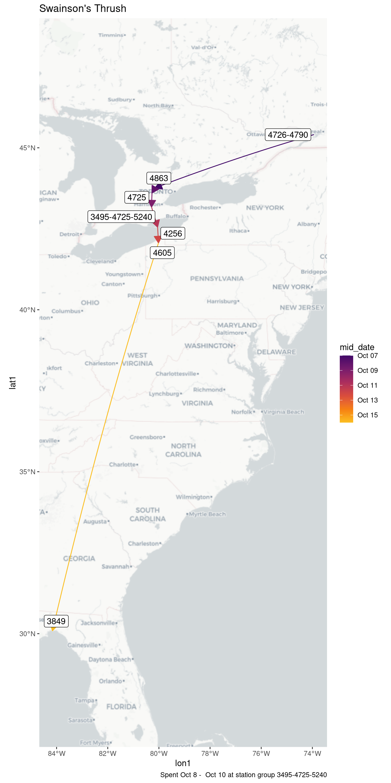
plot_map(trans, 34474) +
  labs(title = "White-throated Sparrow",
       caption = "Spent Oct 19 - Oct 27th at station group 5398-7354")
Zoom: 8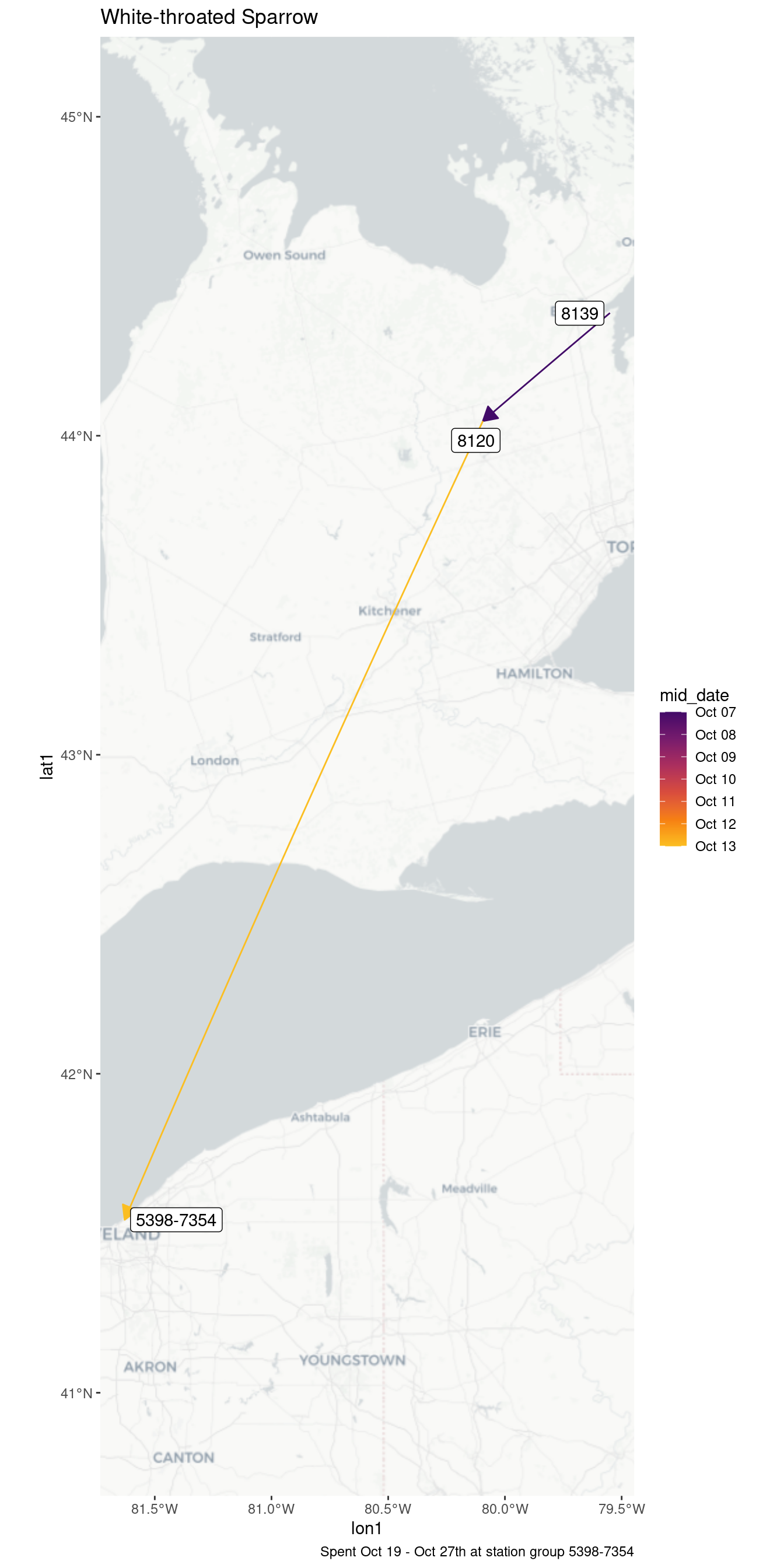
Looking at circadian patterns
Directed exploration
This is a quick look at circadian patterns of movement, especially for in BC birds in the fall.
We first do a quick look to pull out some ids of relevant birds to explore. Then we create start and end columns to hold the hour of day values (i.e. 10.5 which would be 10:30 am, local time).
# To find birds in BC which have many records
b <- filter(bouts_split, recvDeployLon < -110, recvDeployLat > 48.97) |>
summarize(n = n(), .by = c("tagDeployID", "english")) |>
arrange(desc(n))
# To convert start times to start/end fractional hours (i.e. time of day rather than date/time)
b0 <- bouts_split |>
mutate(start = hour(timeBeginLocal) + minute(timeBeginLocal)/60,
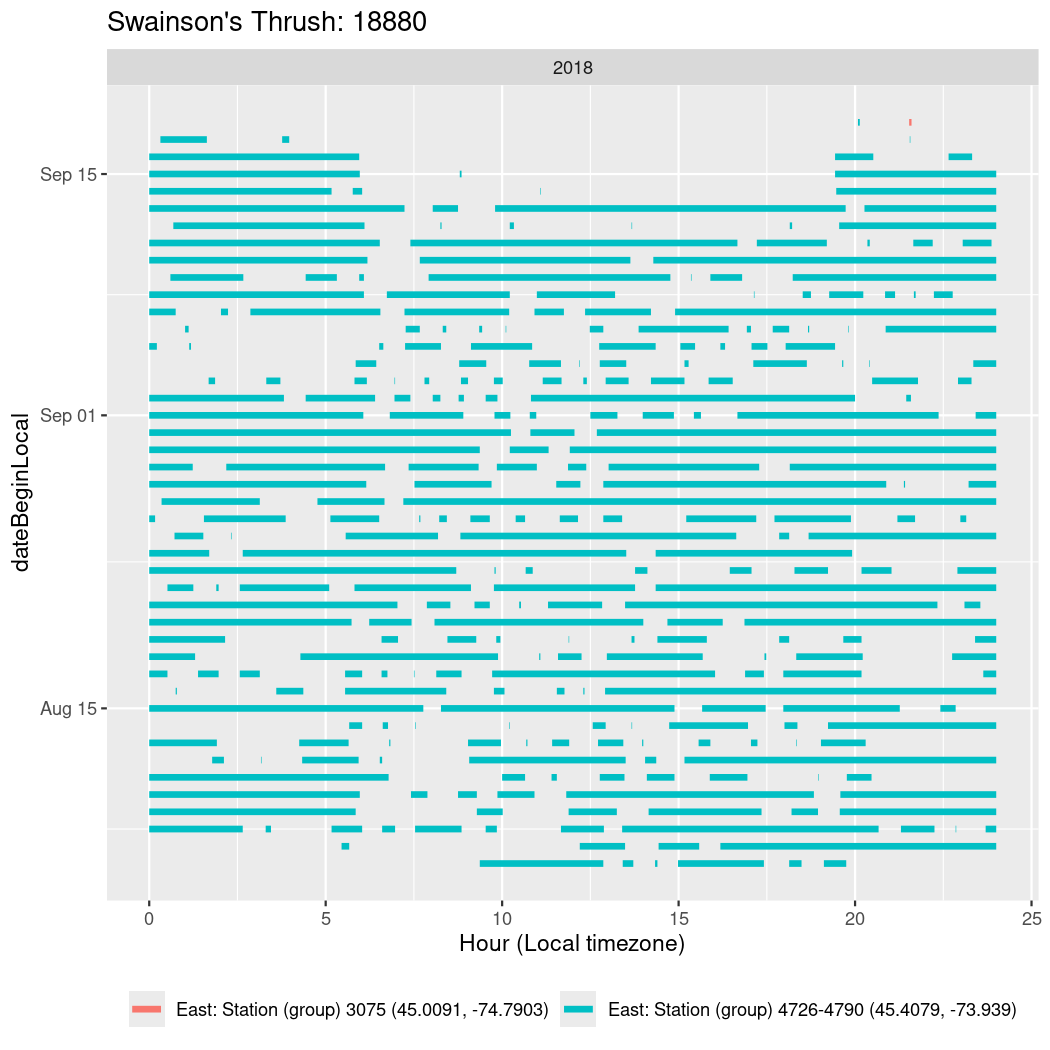
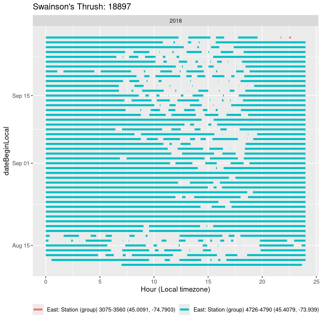
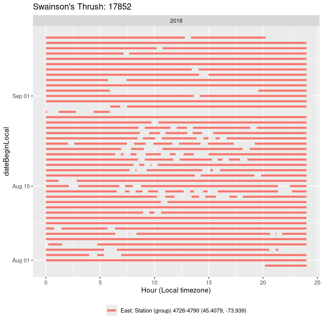
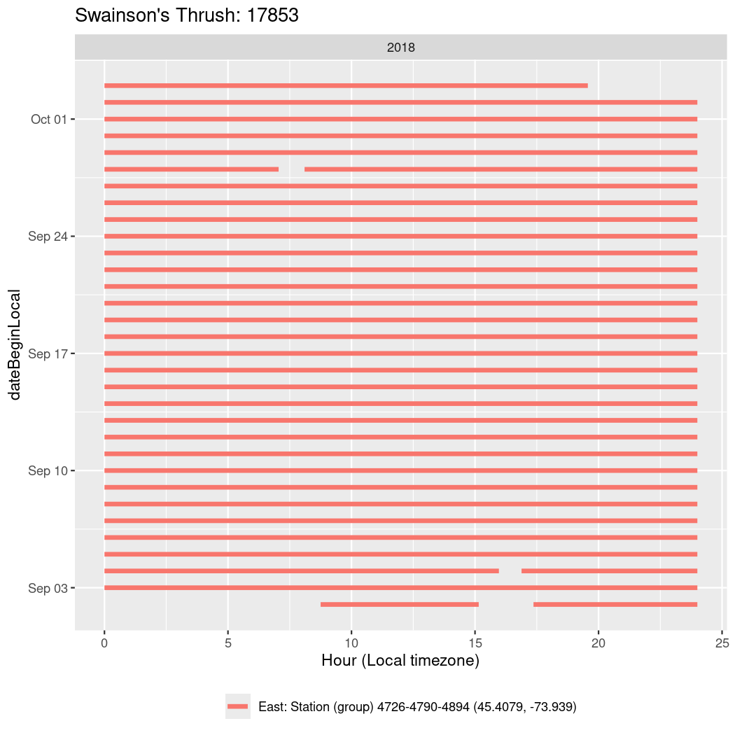
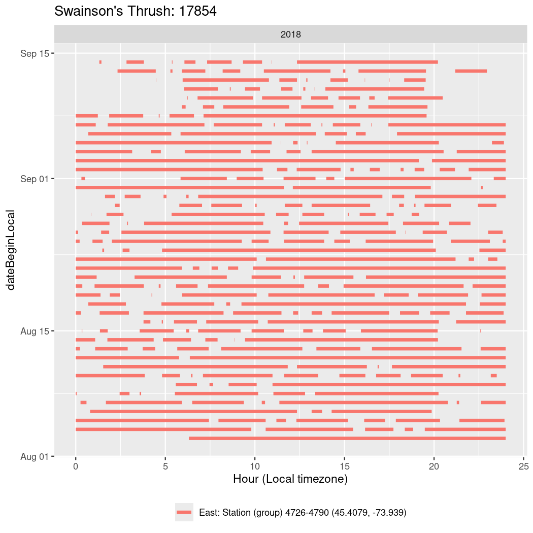
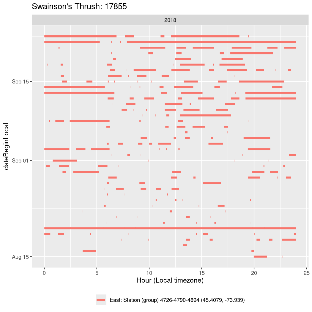
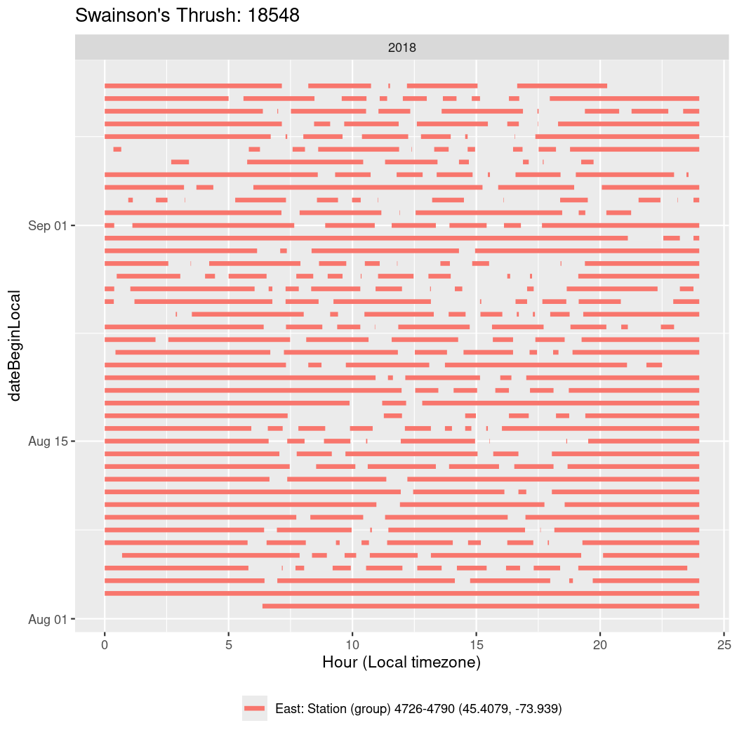
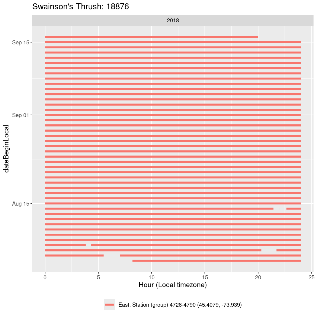
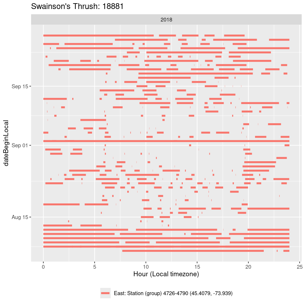
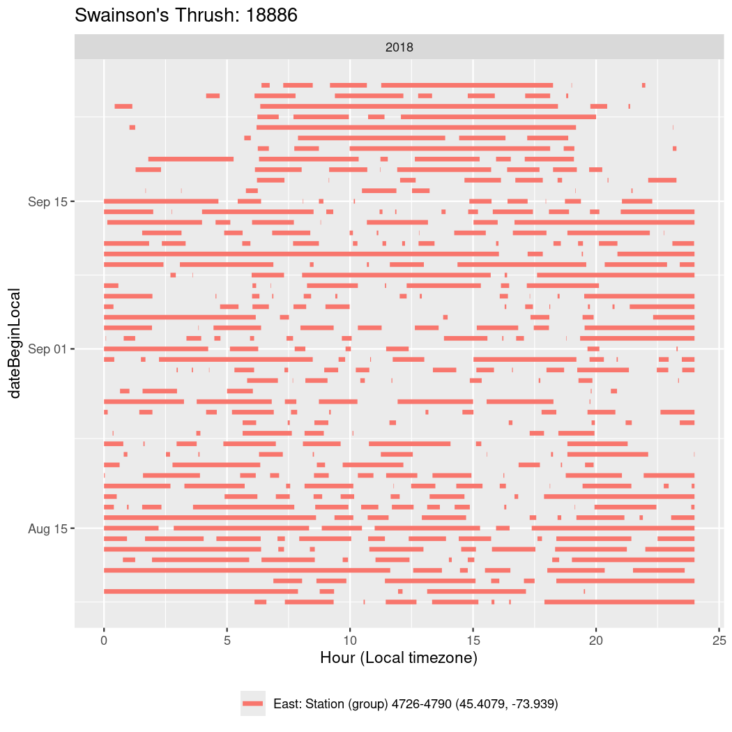
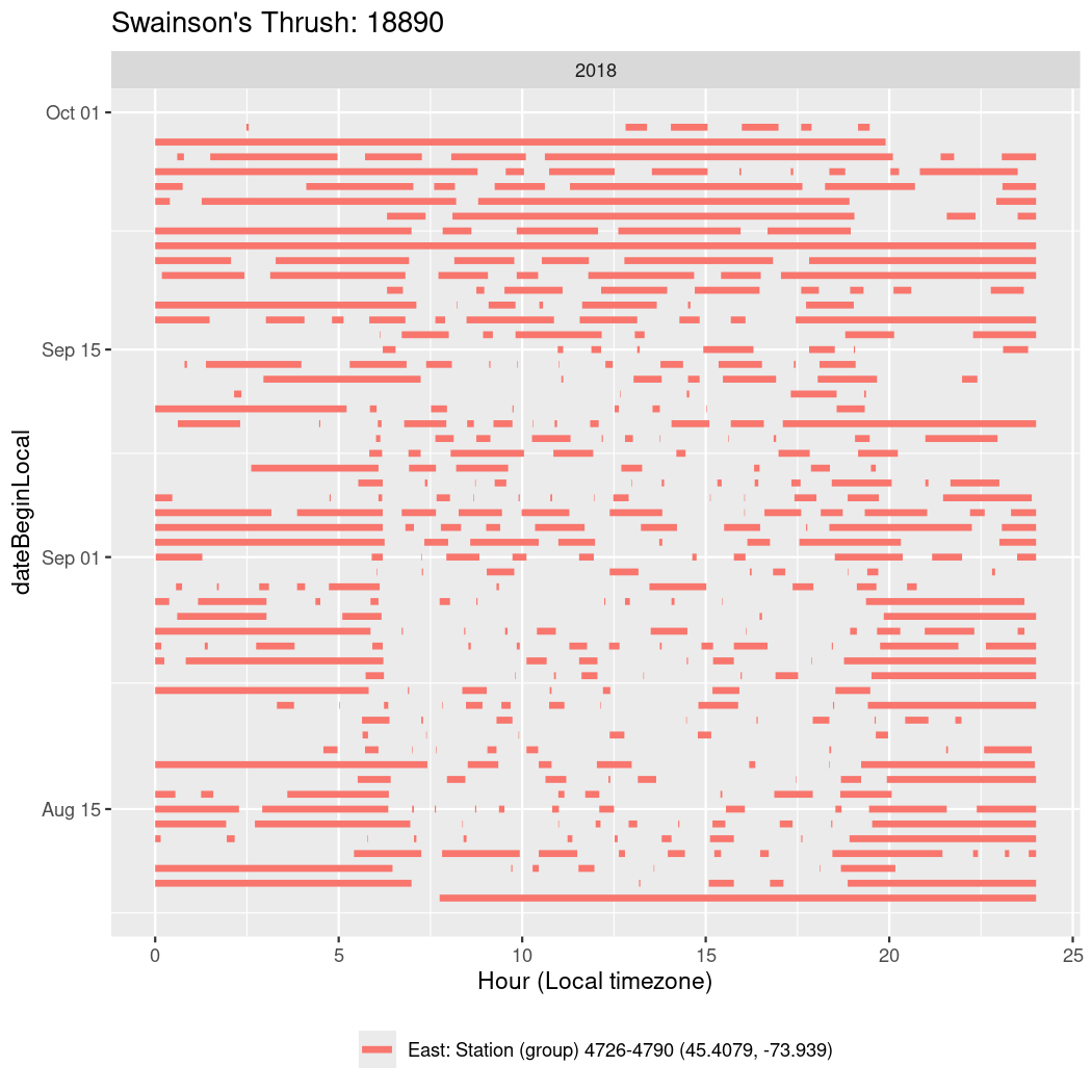
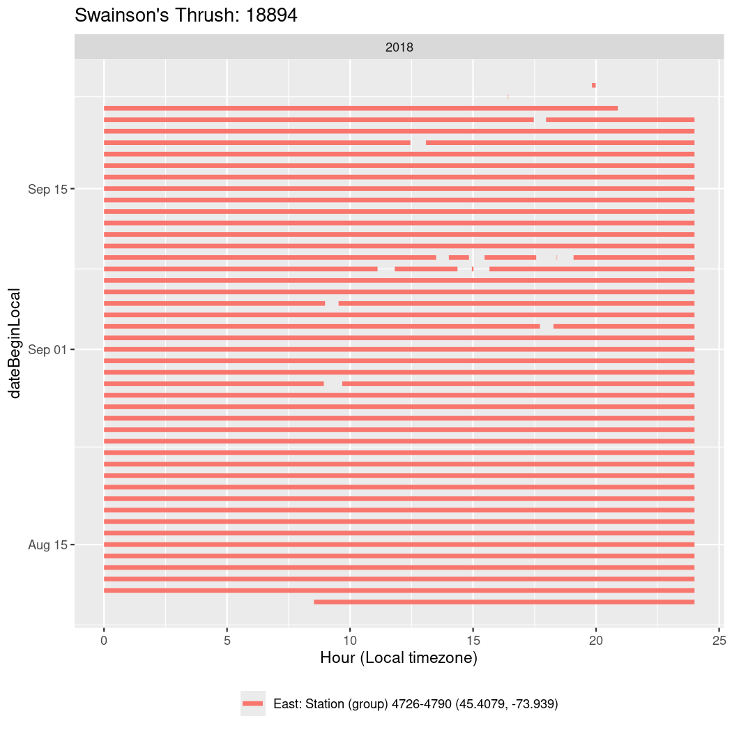
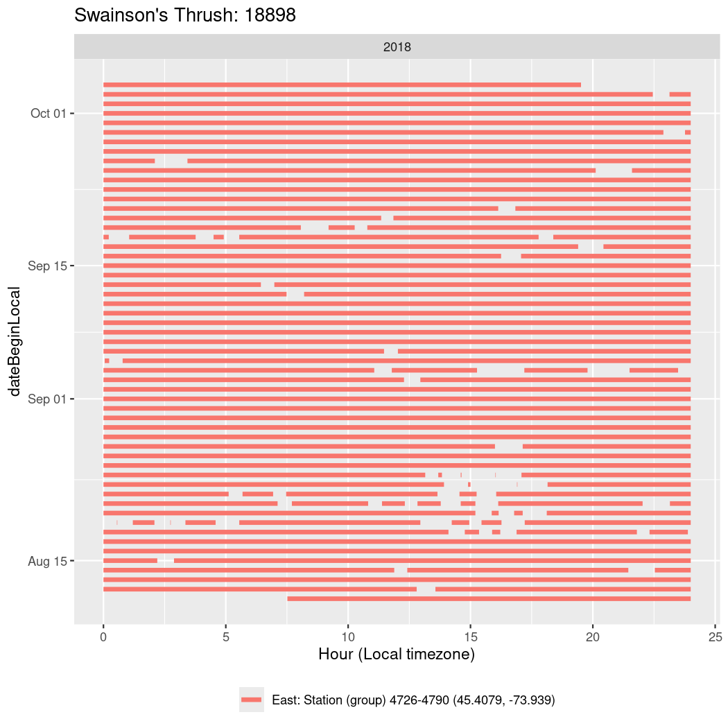
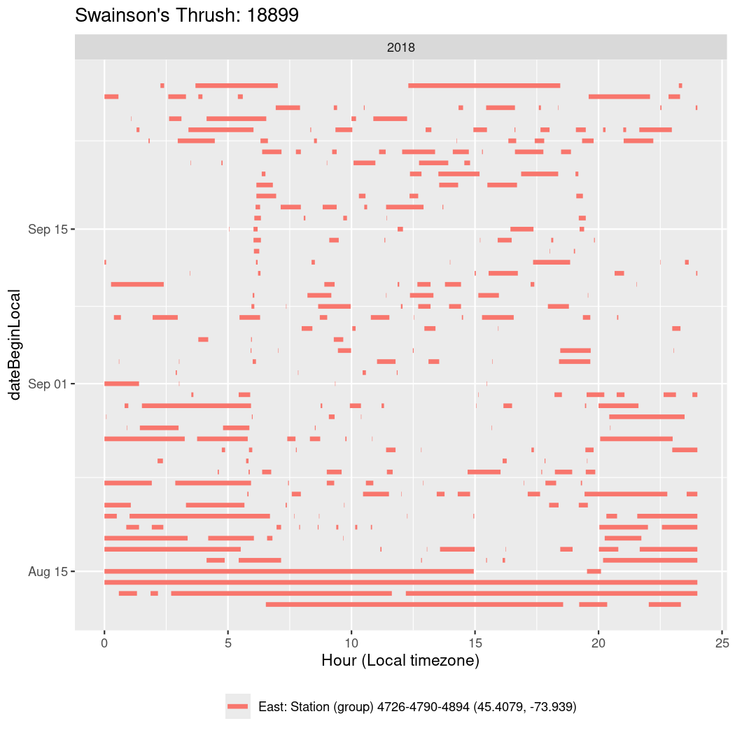
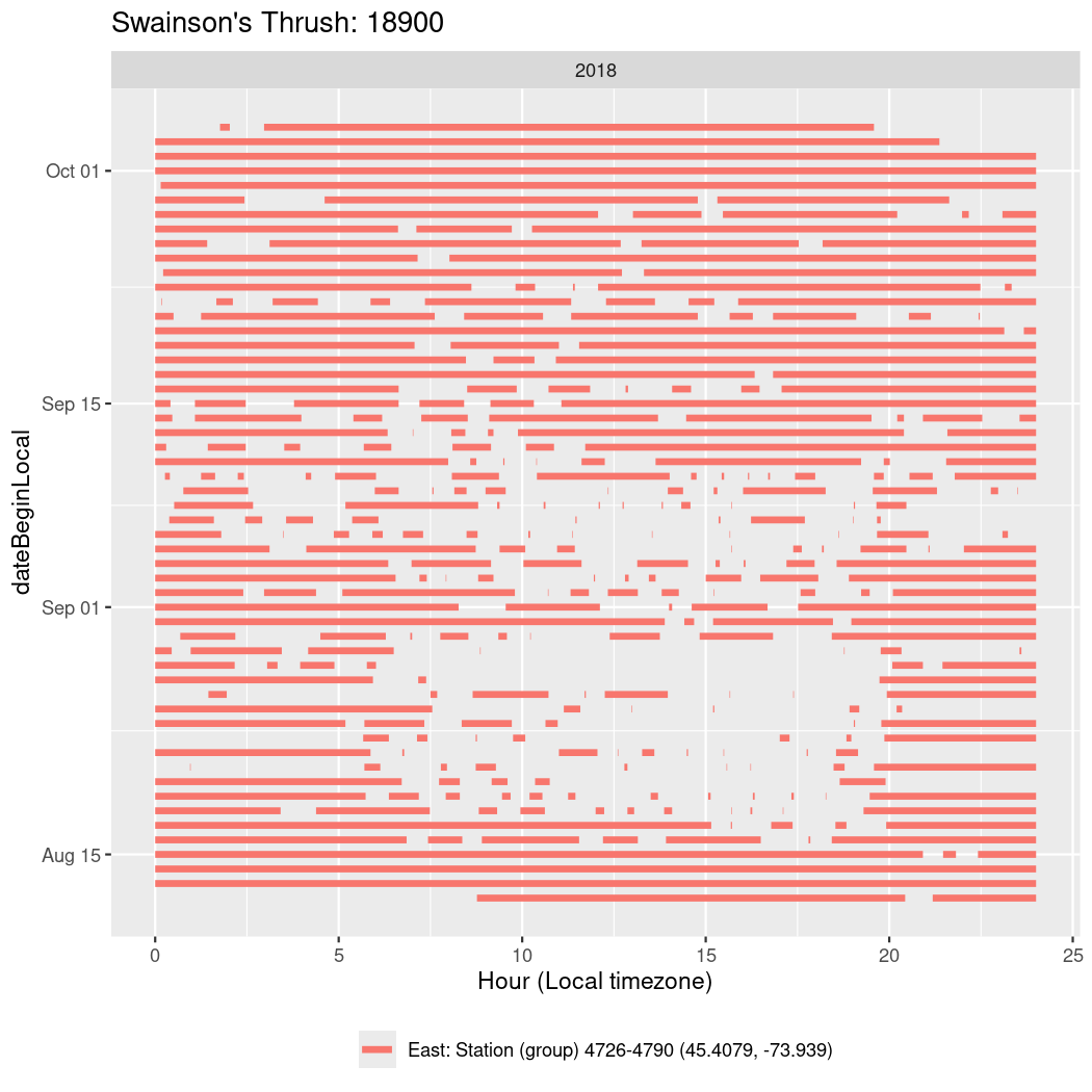
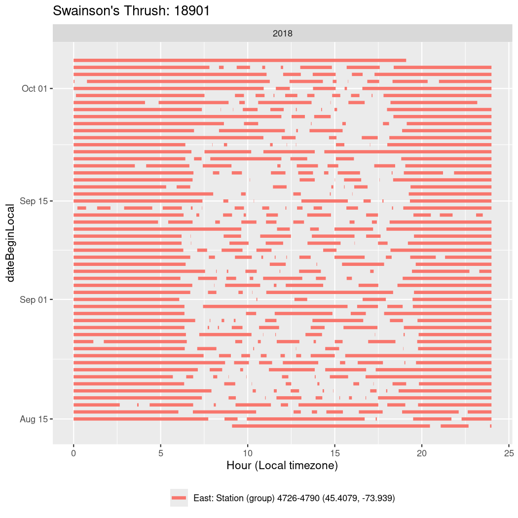
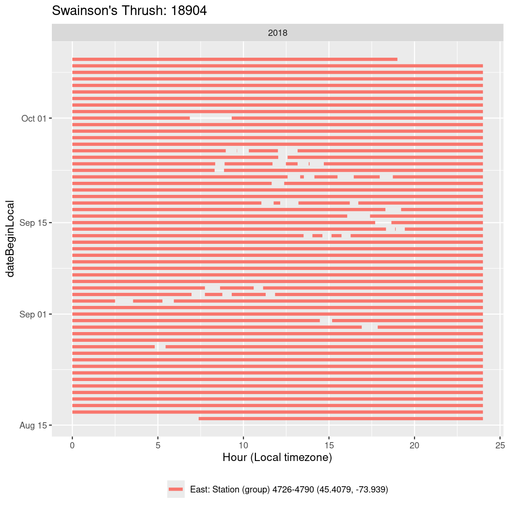
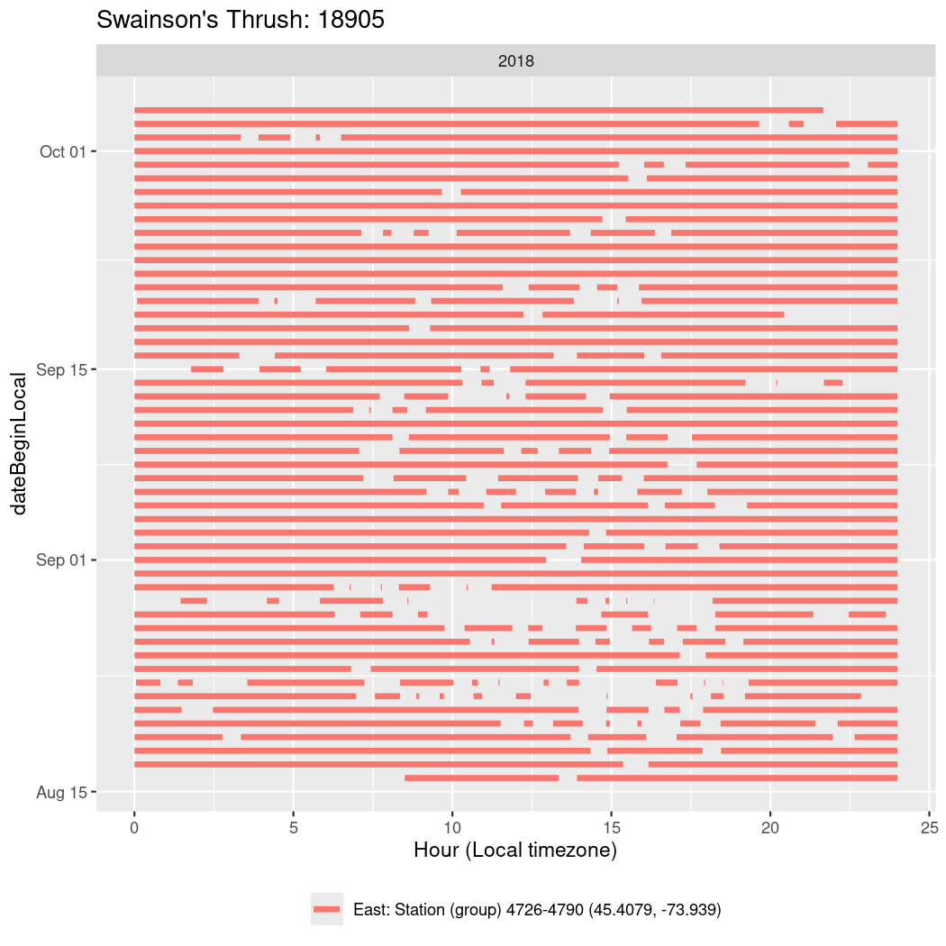
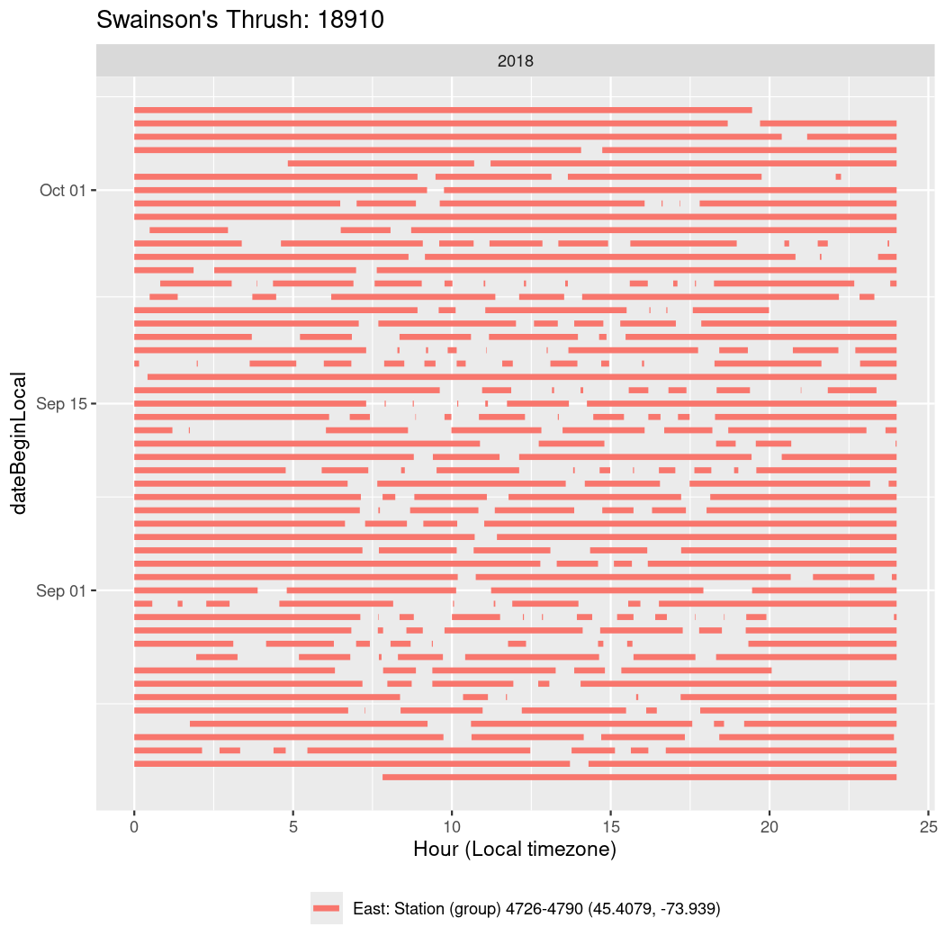
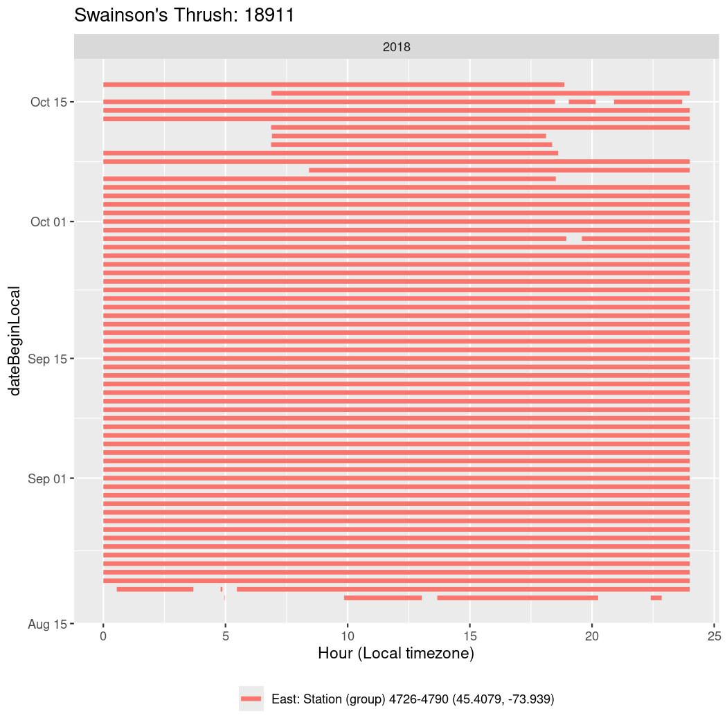
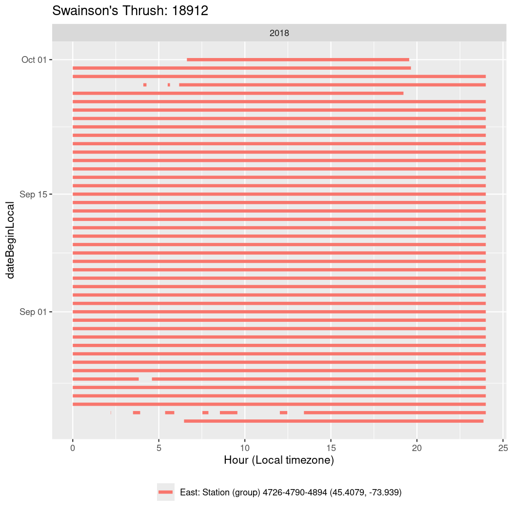
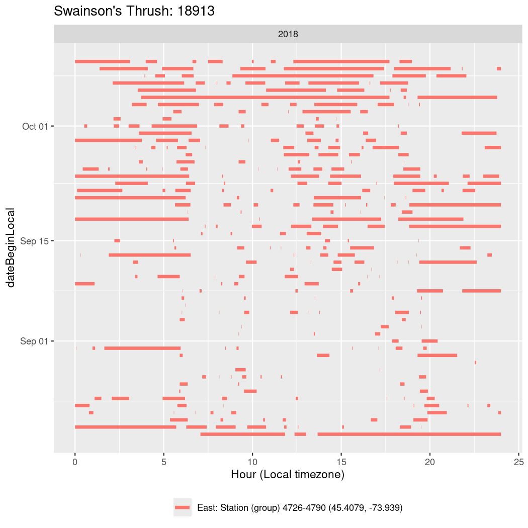
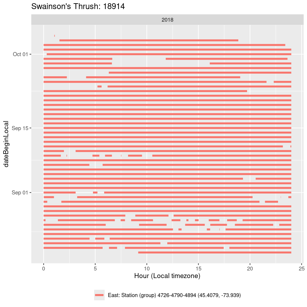
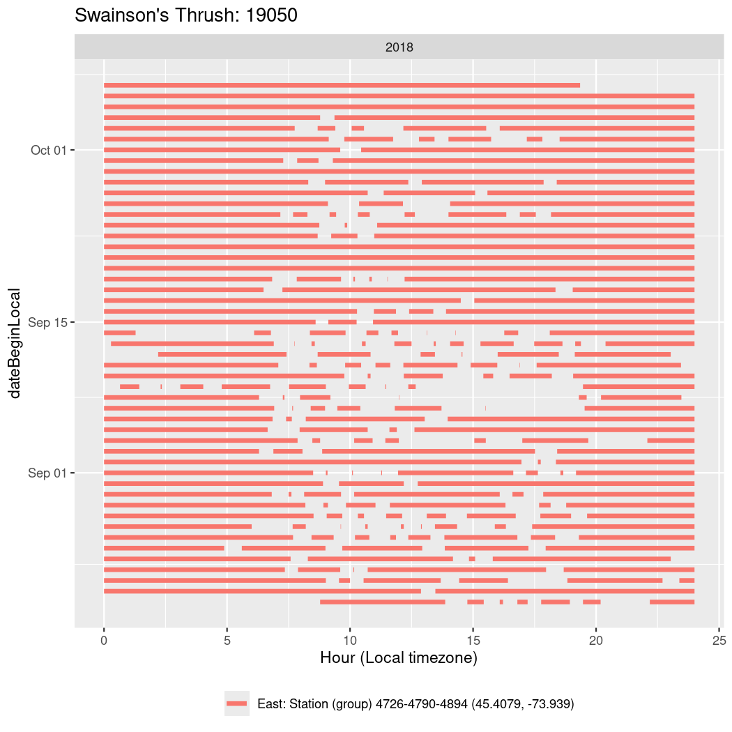
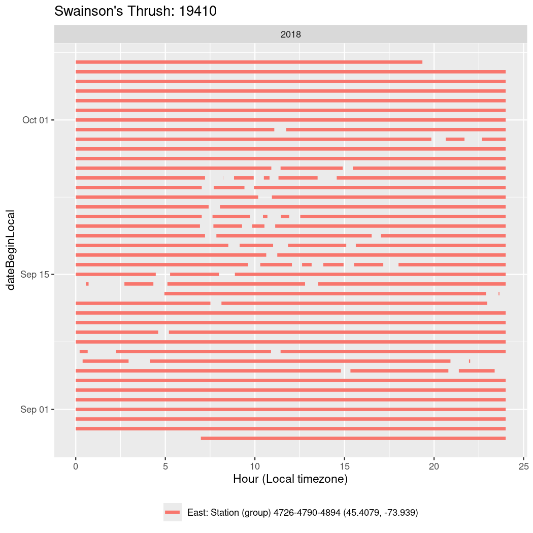
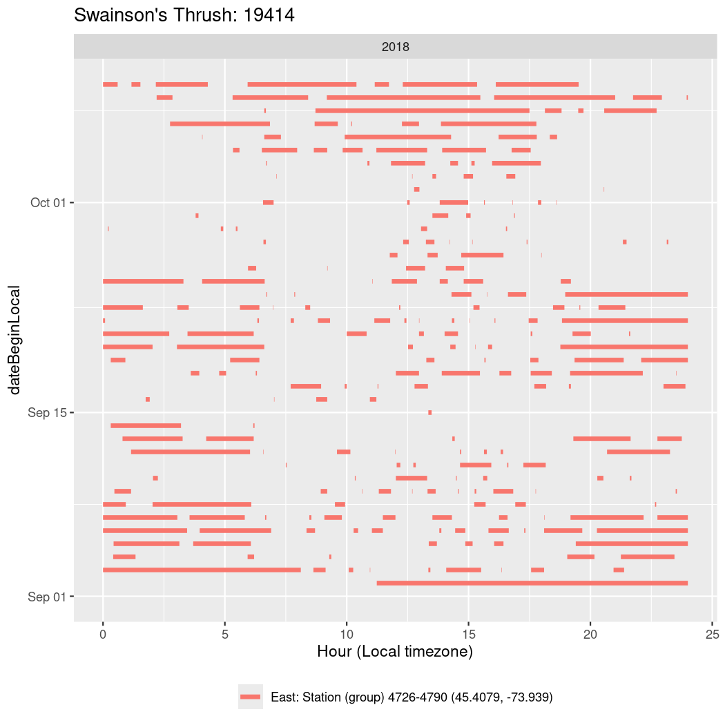
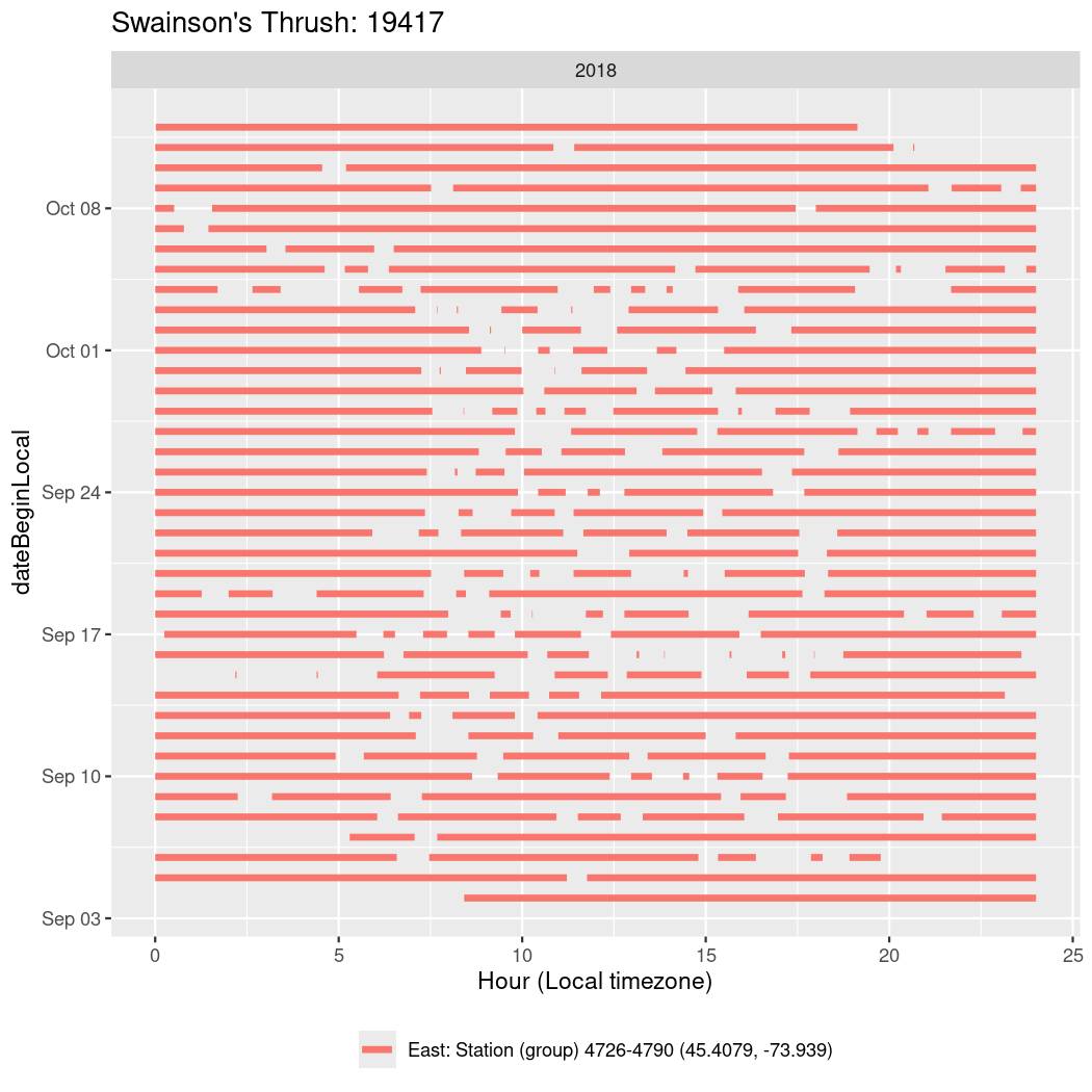
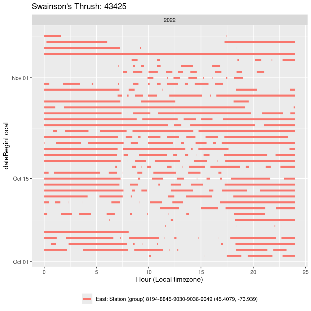
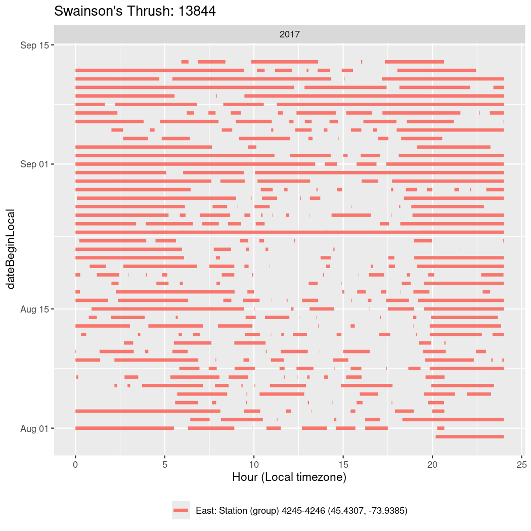
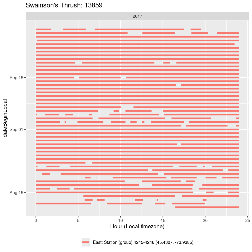
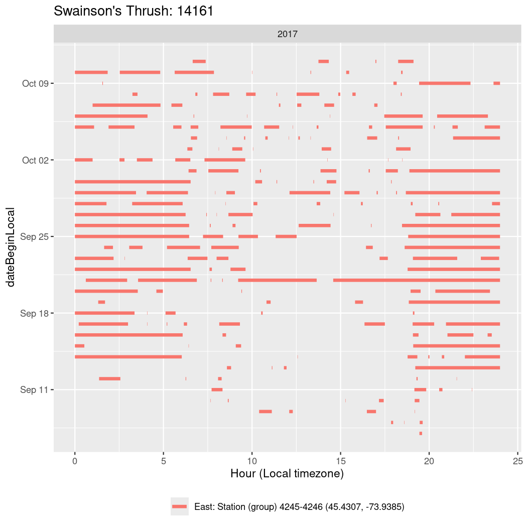
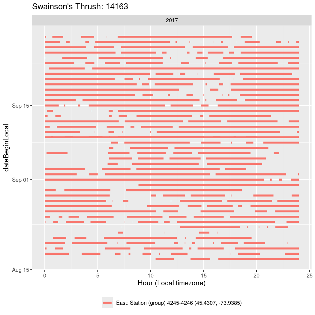
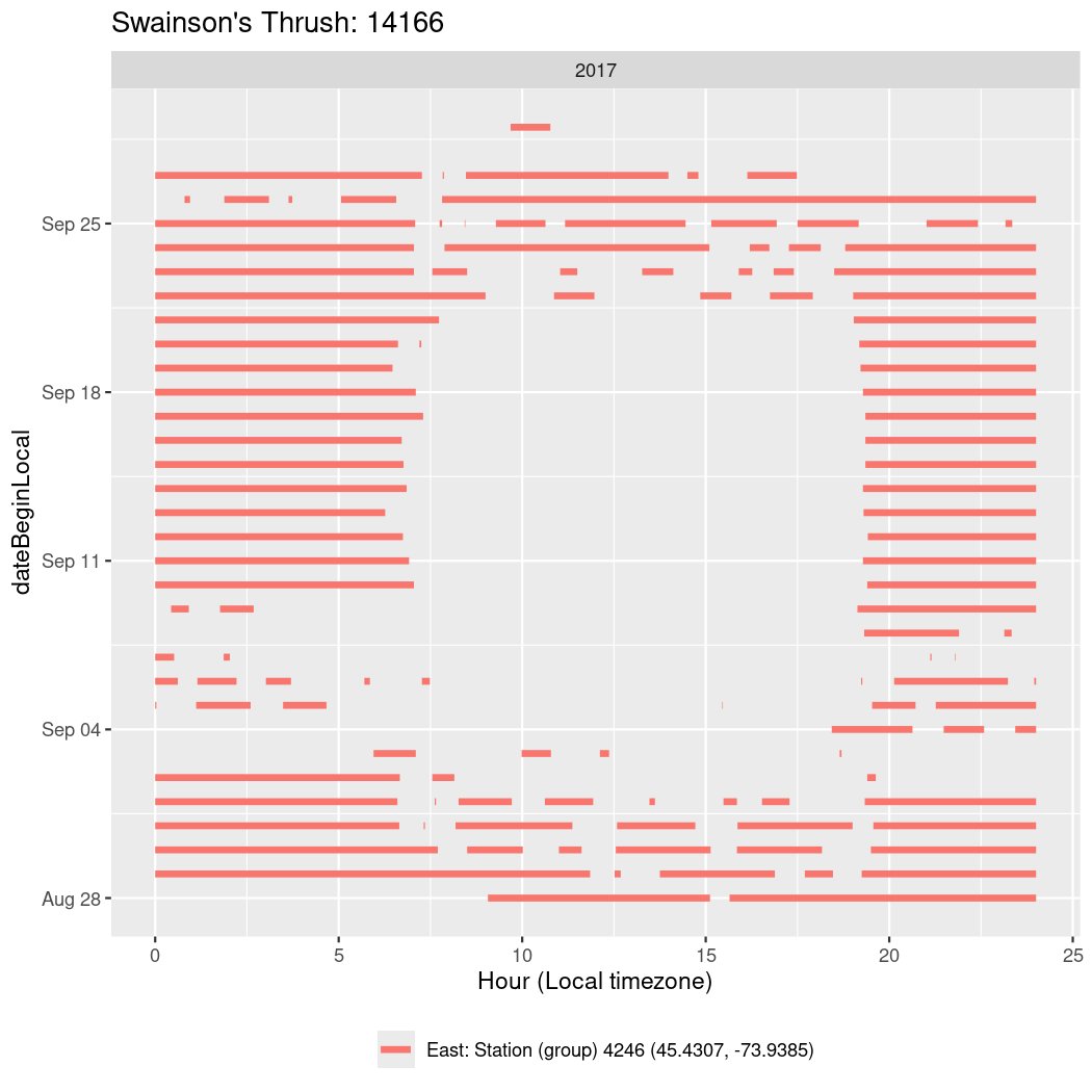
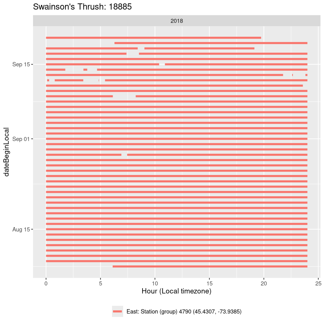
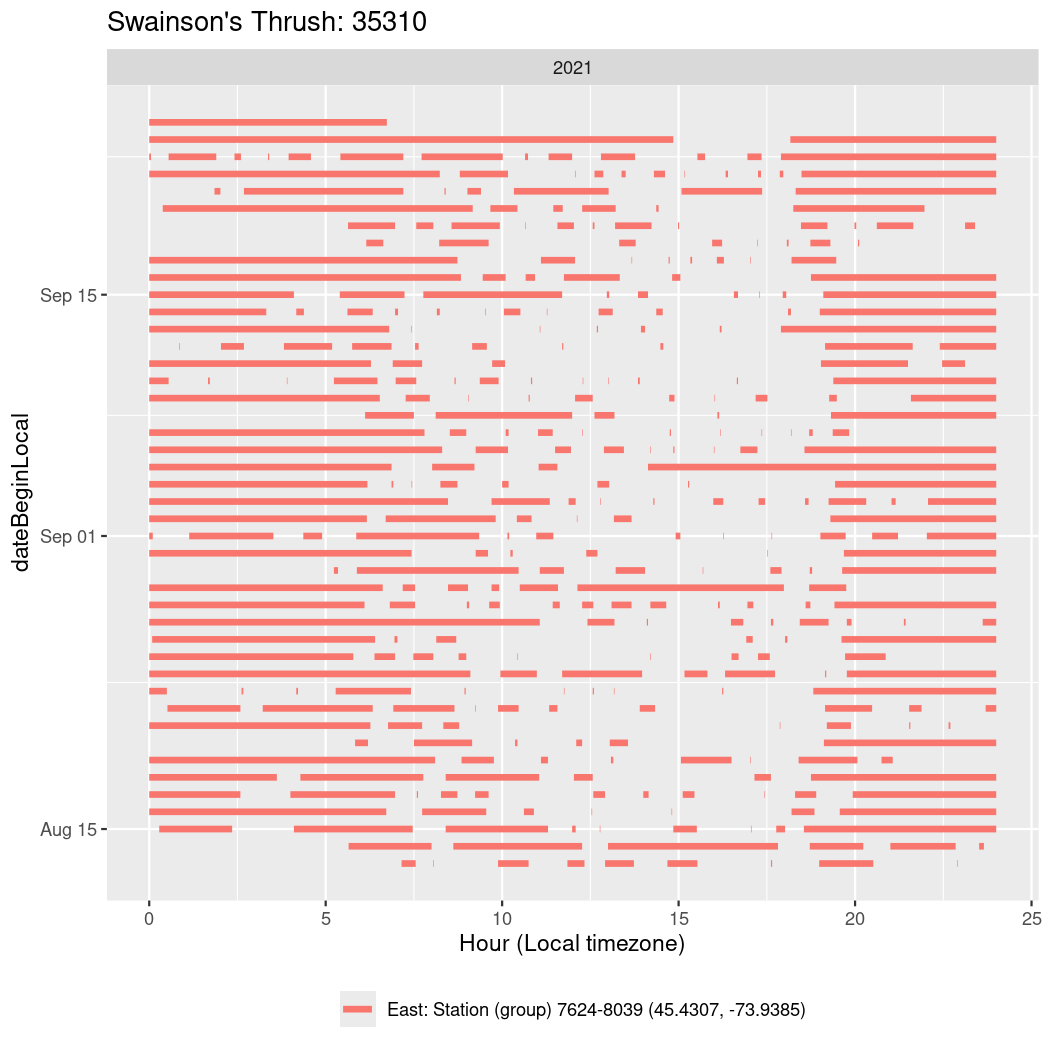
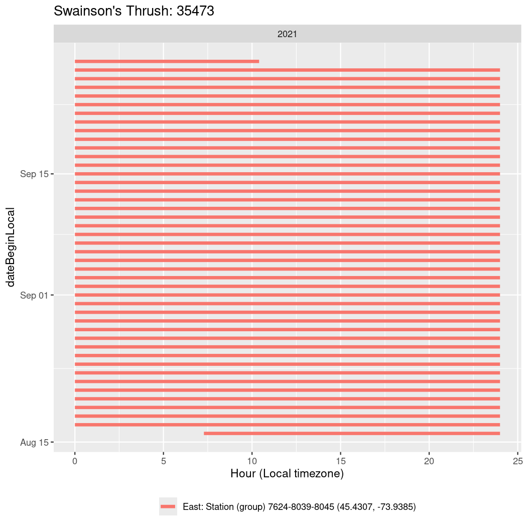
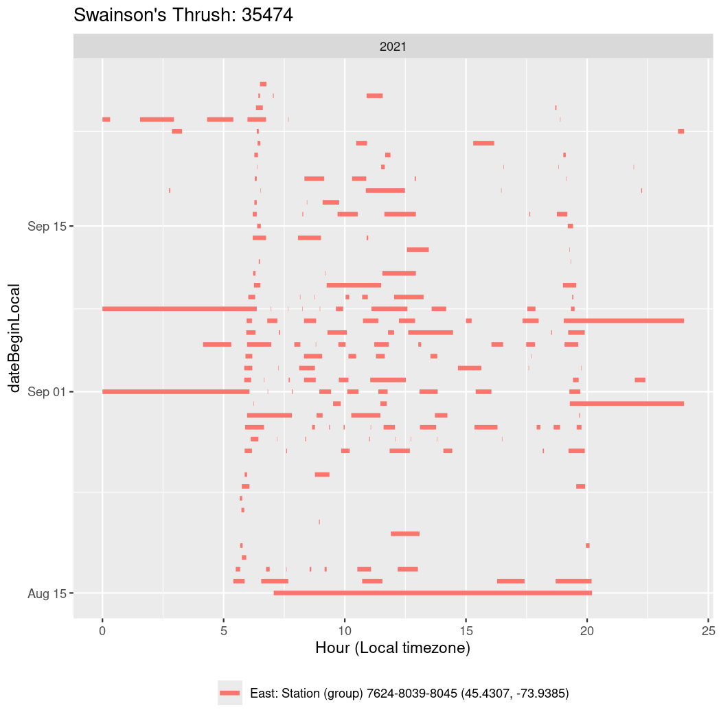
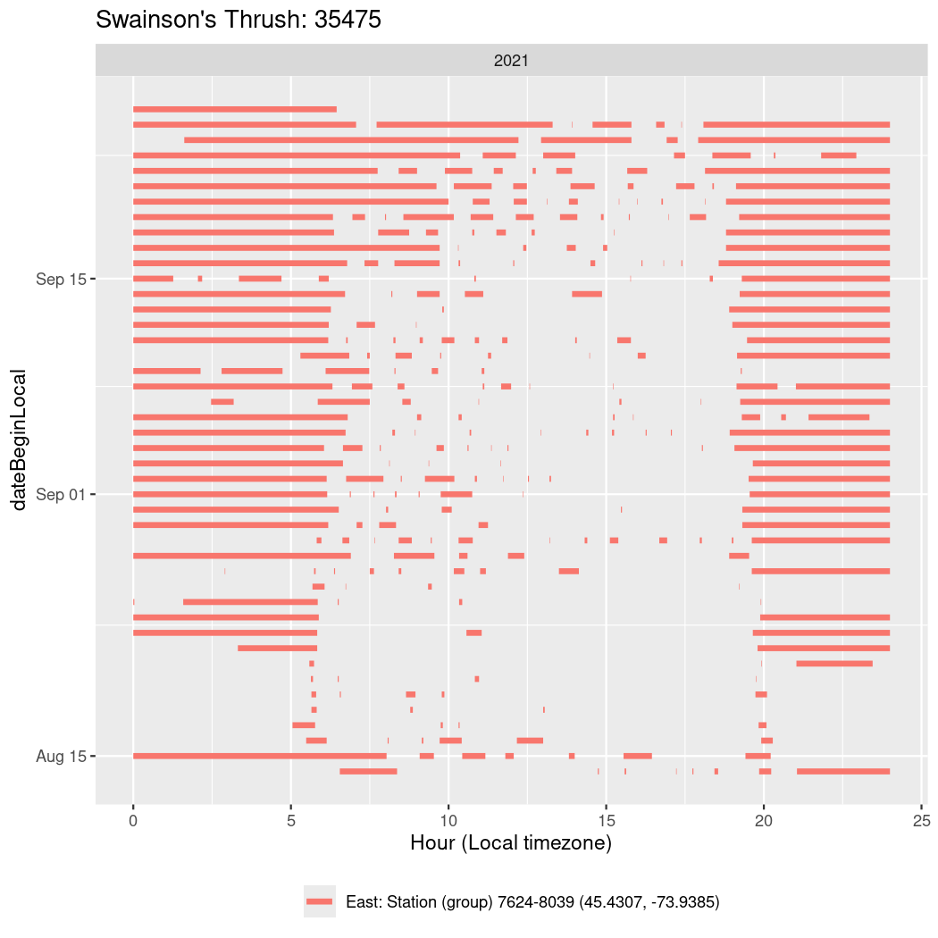
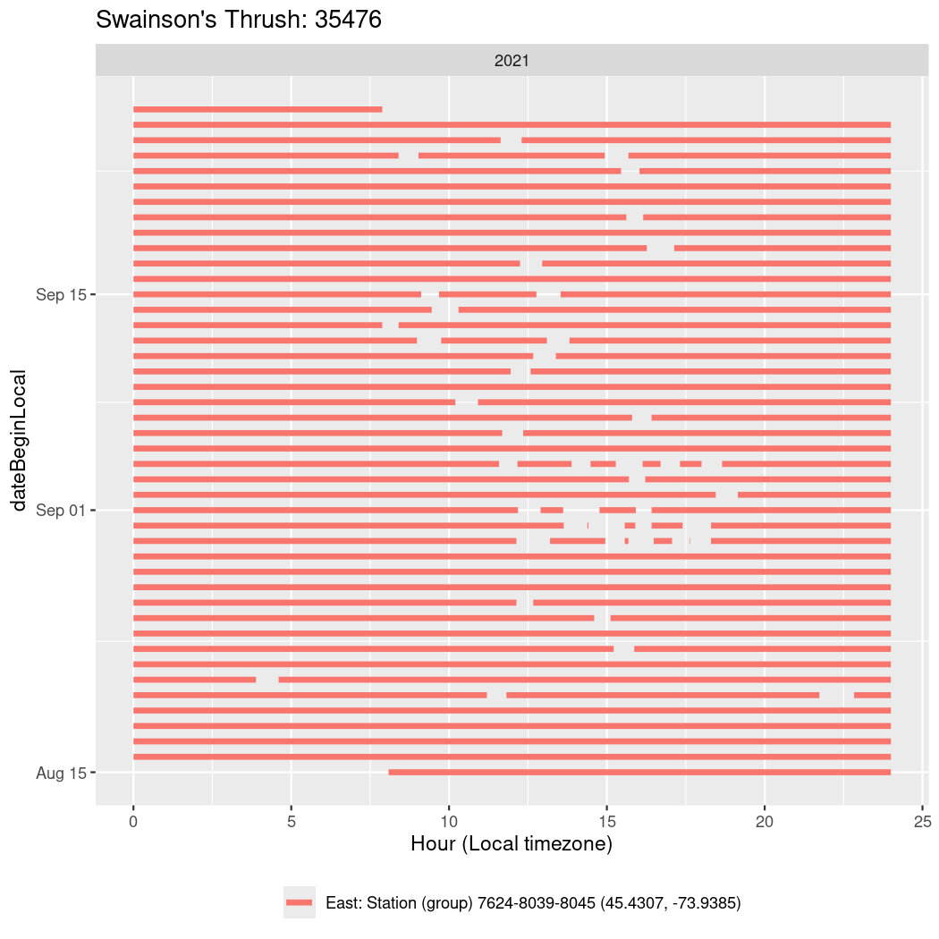
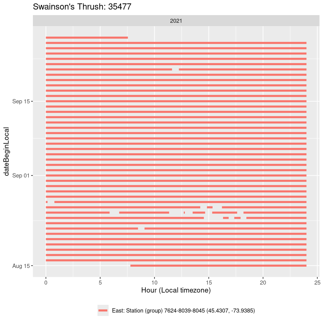
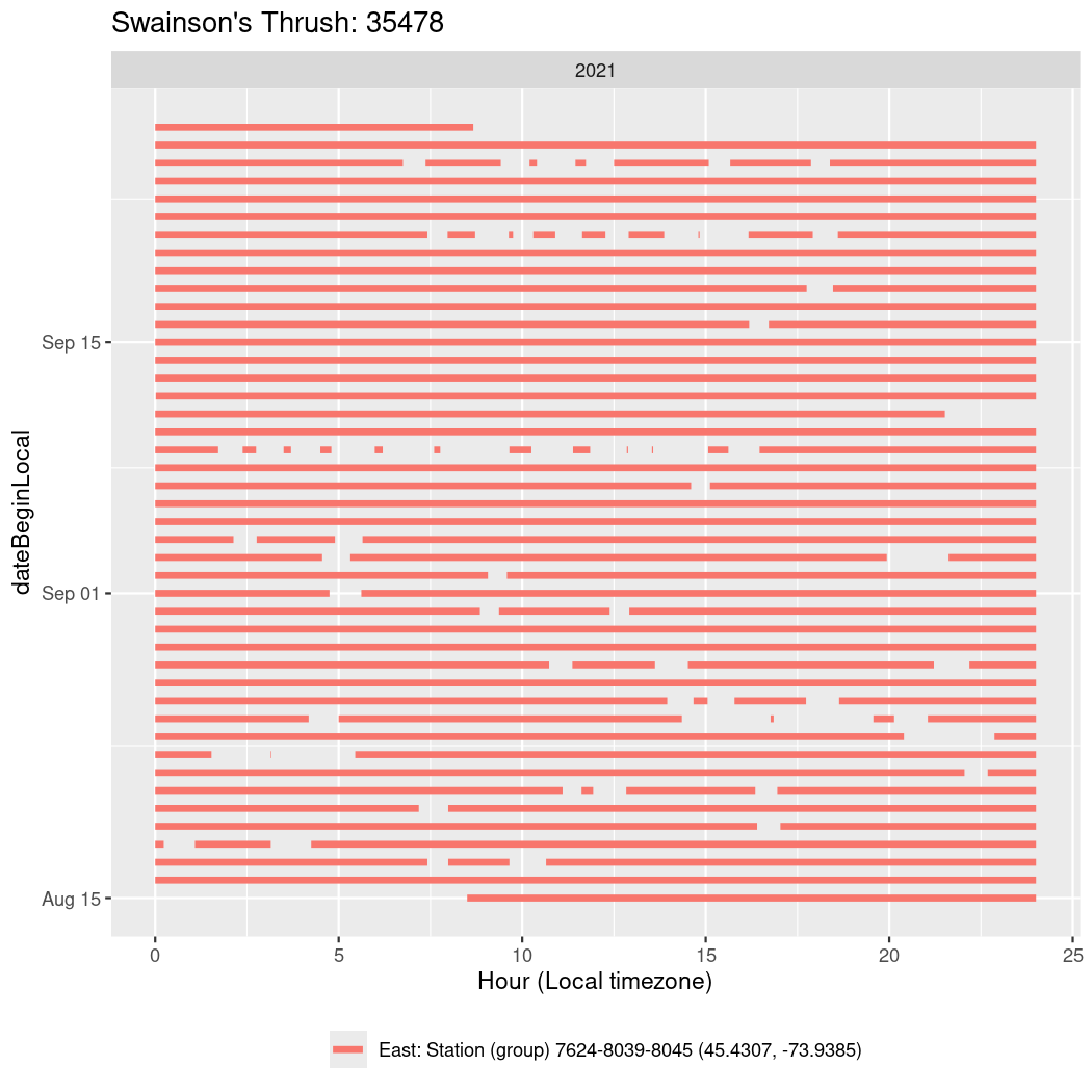
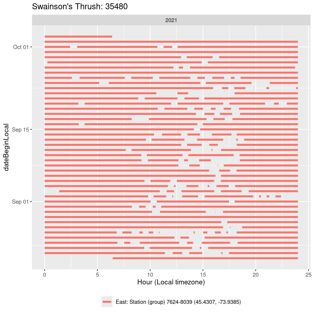
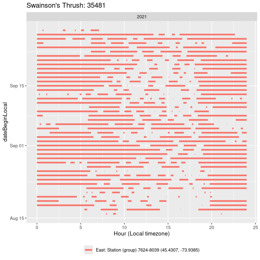
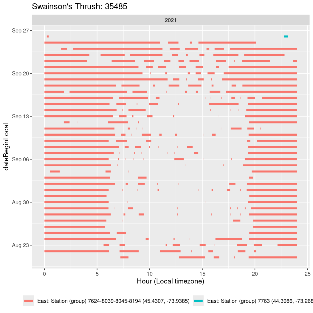
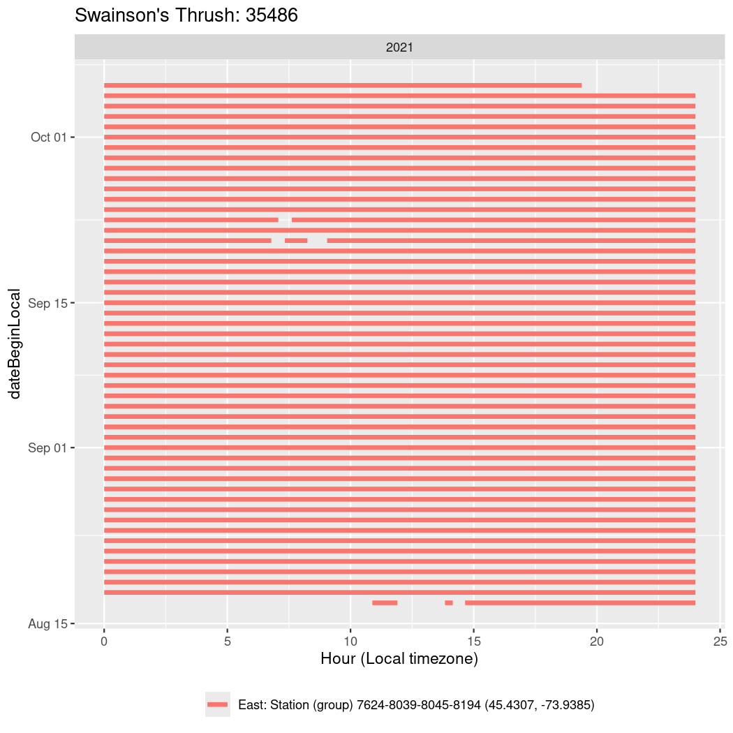
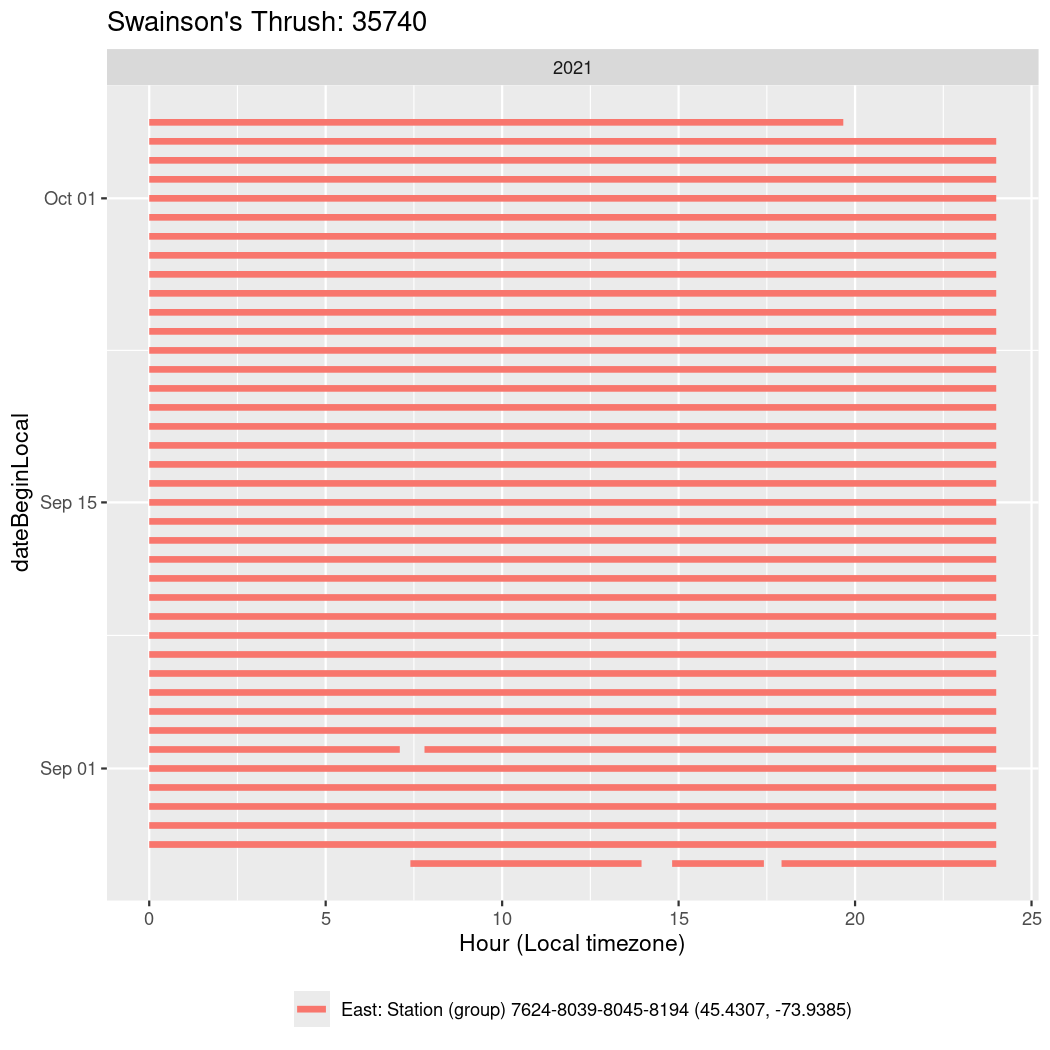
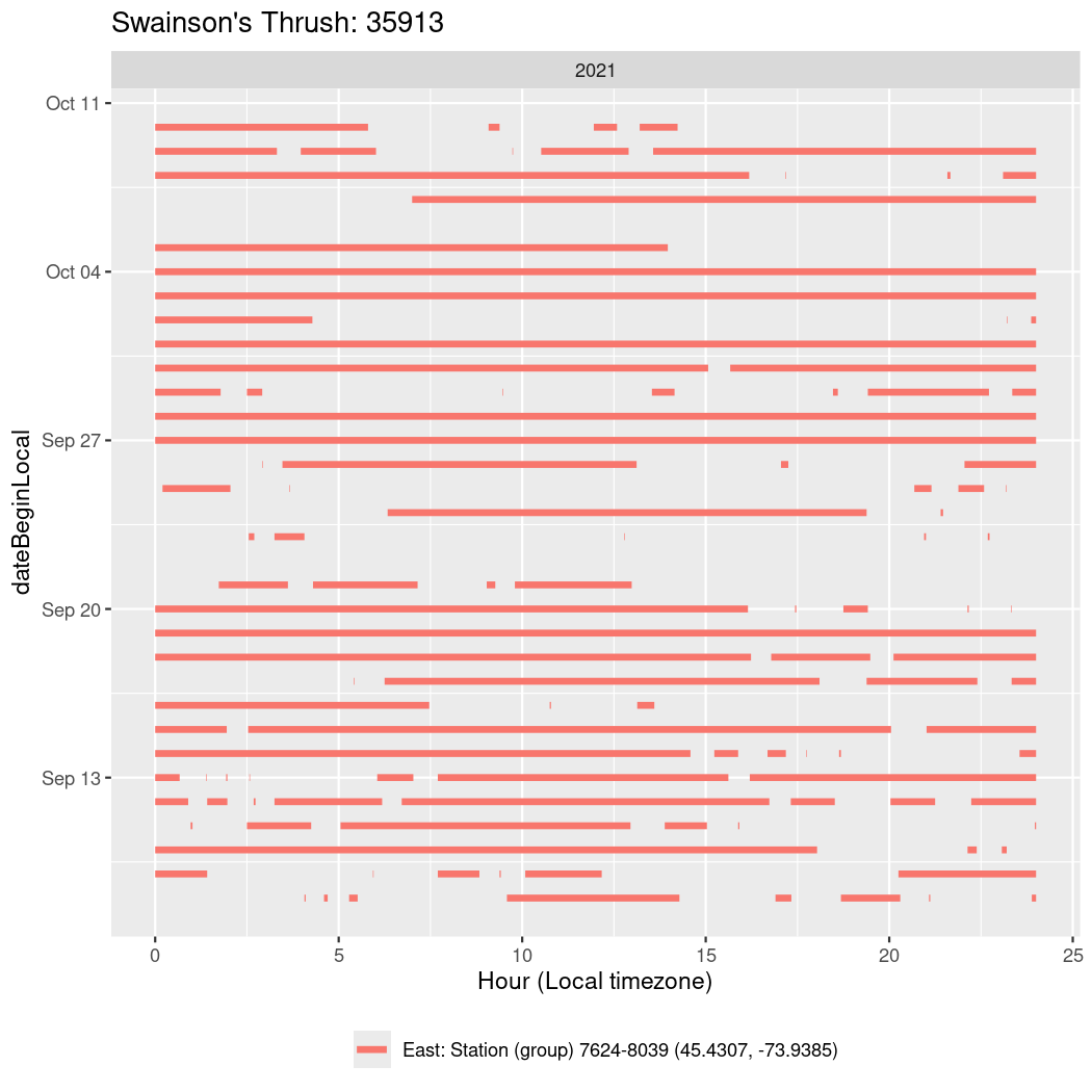
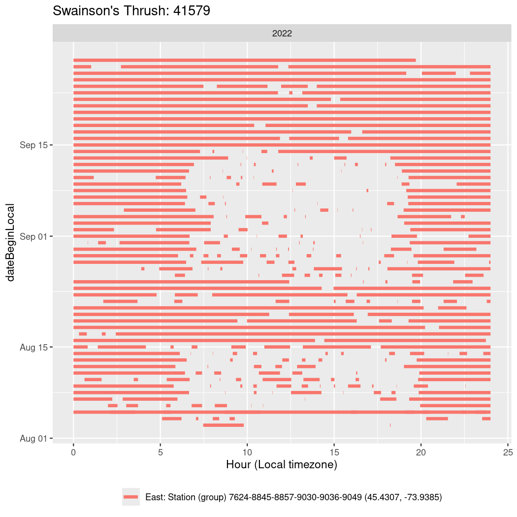
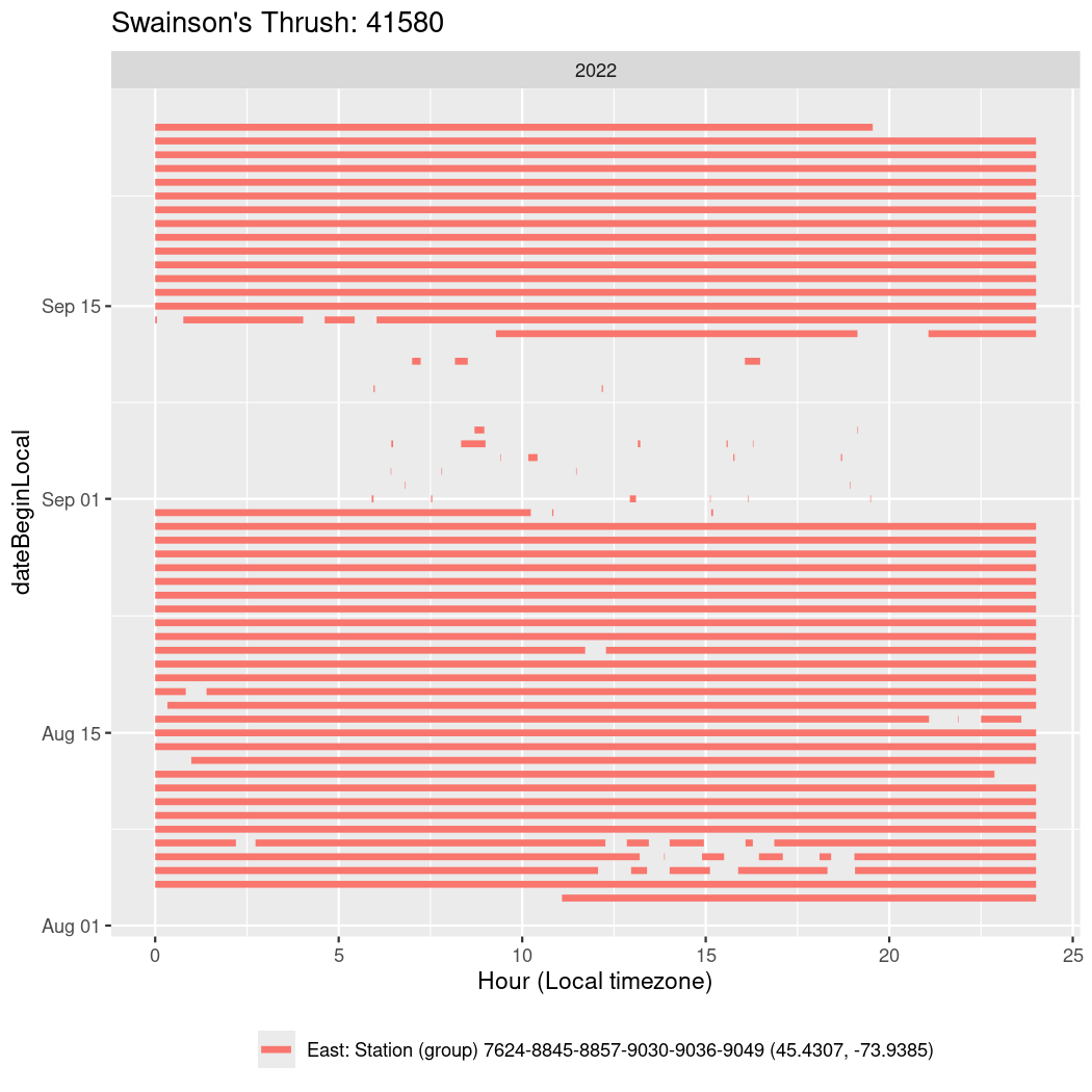
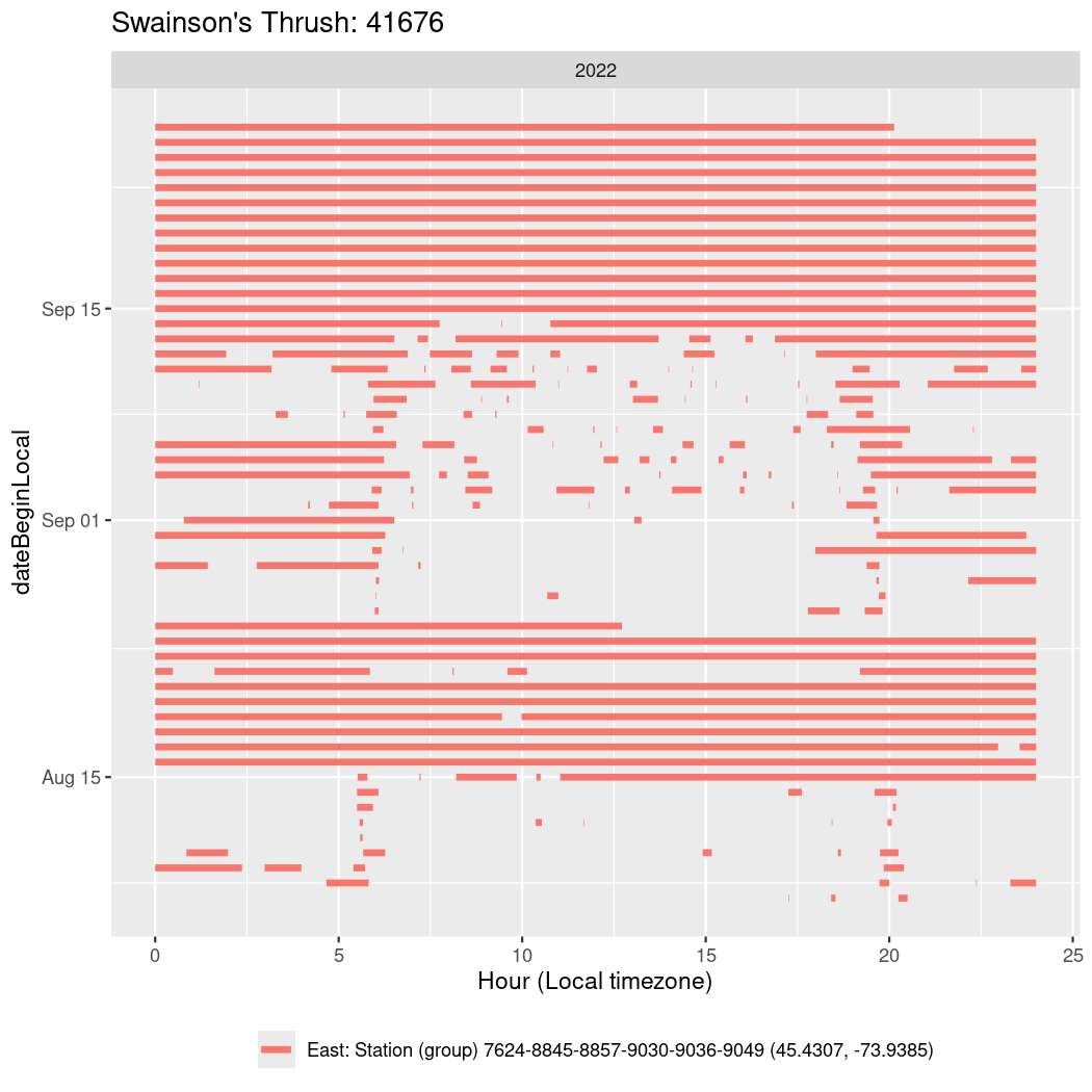
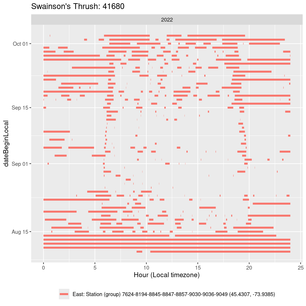
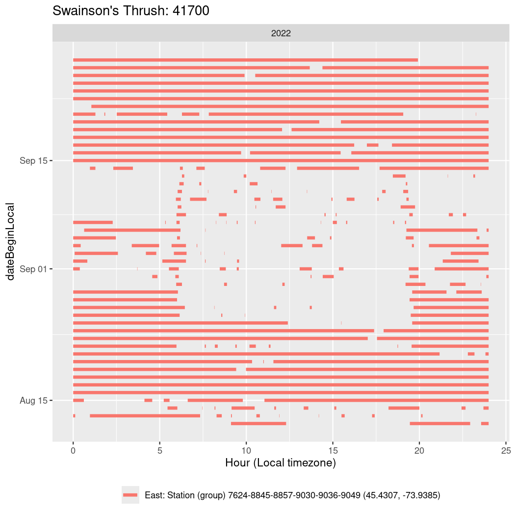
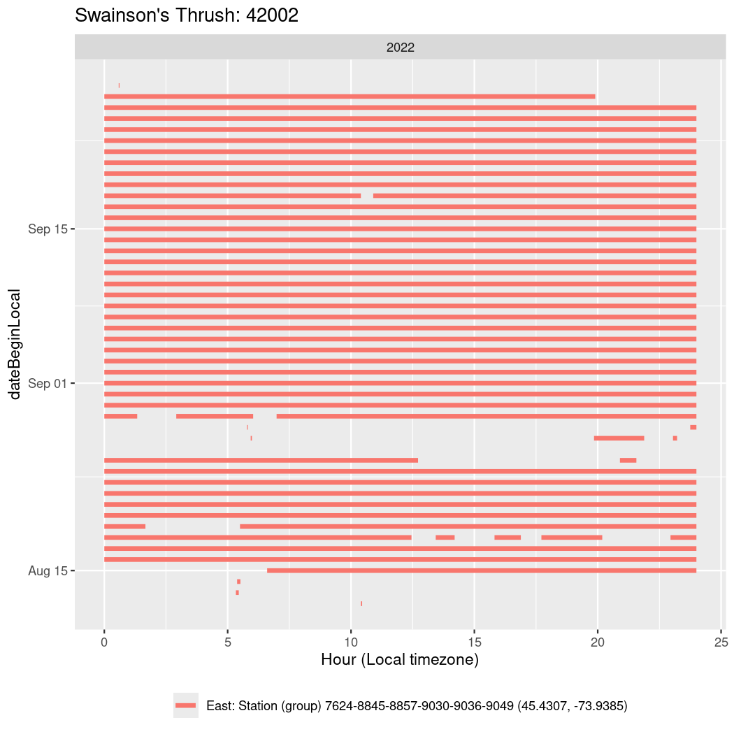
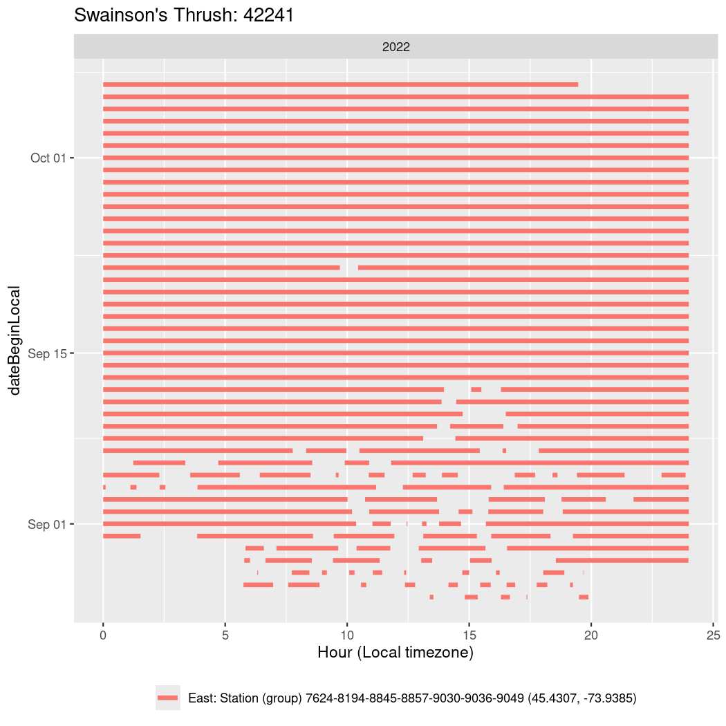
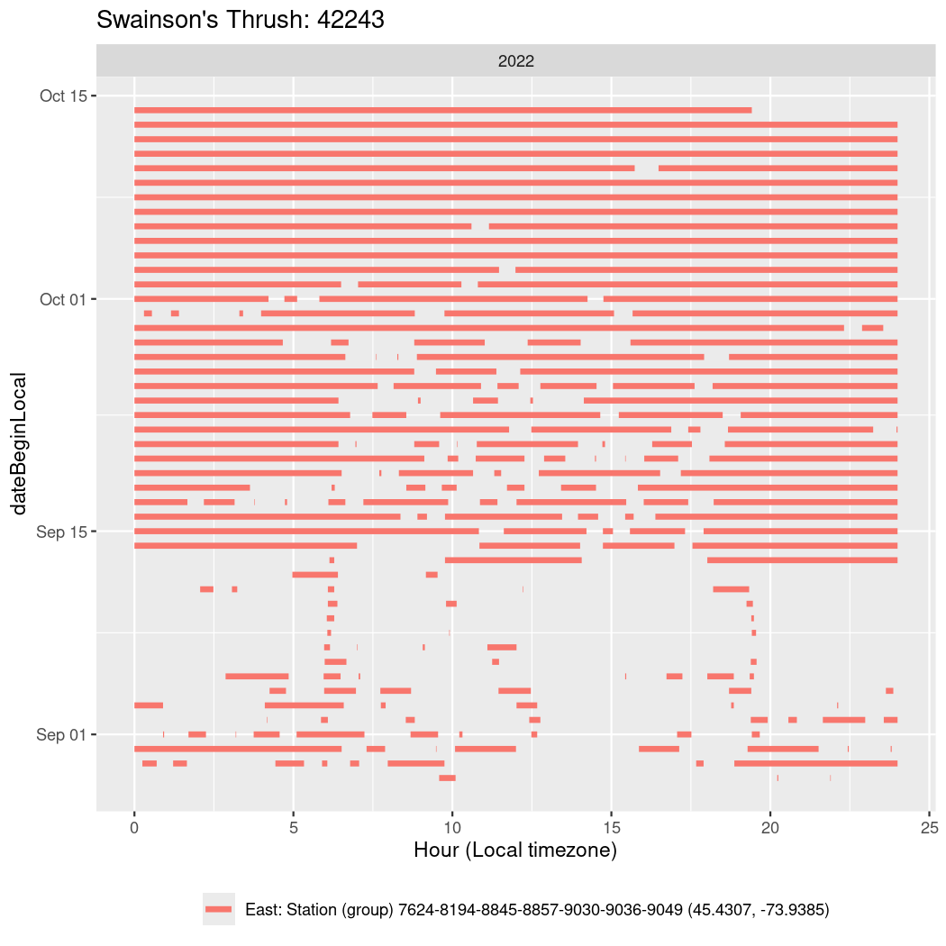
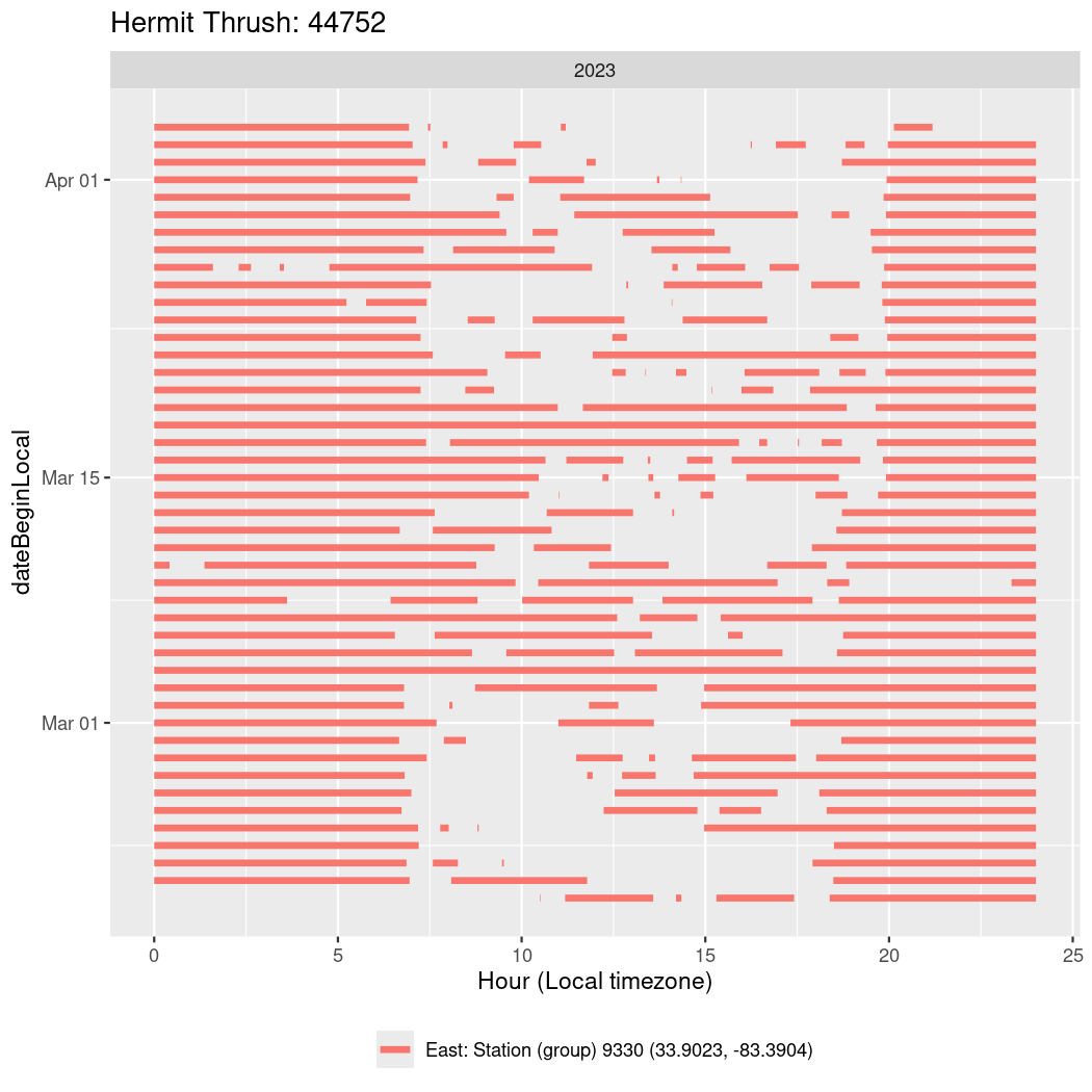
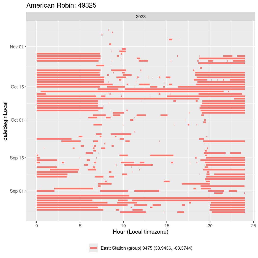
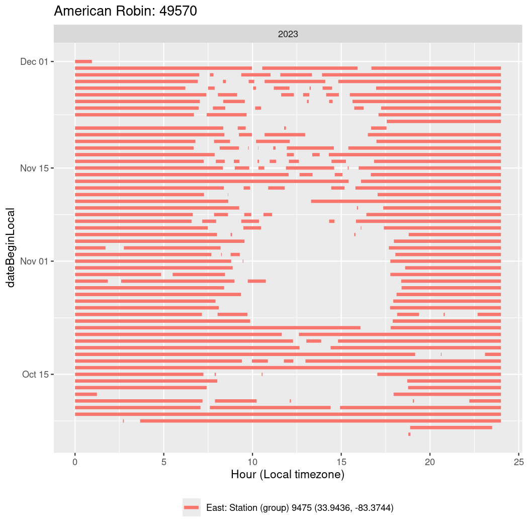
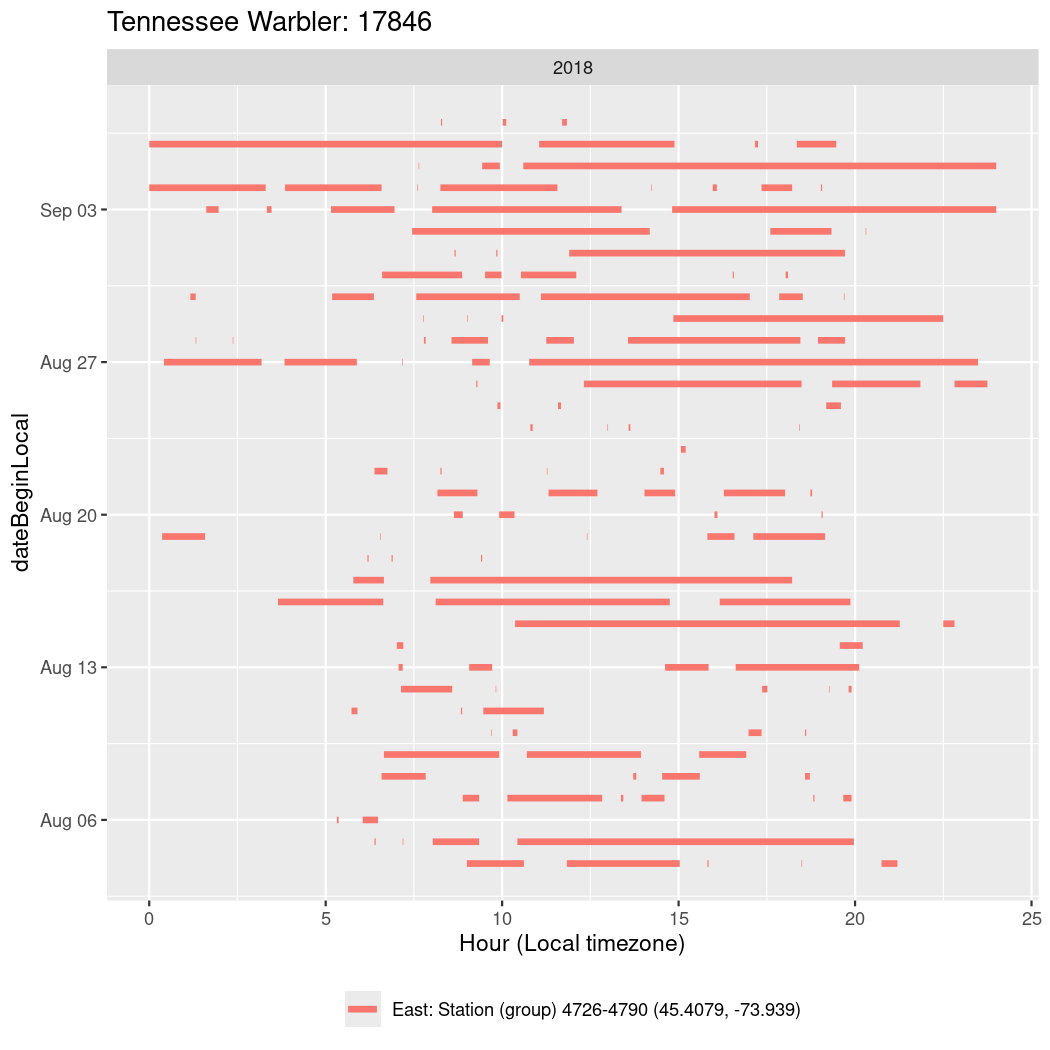
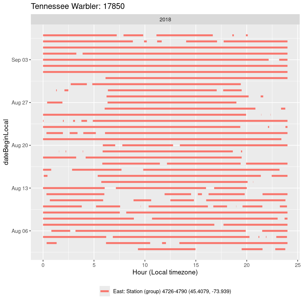
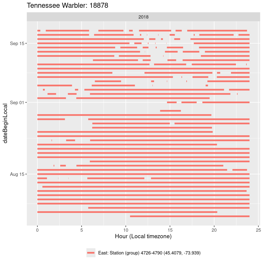
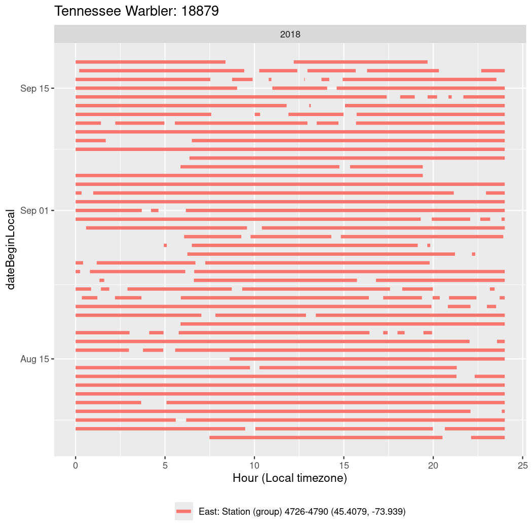
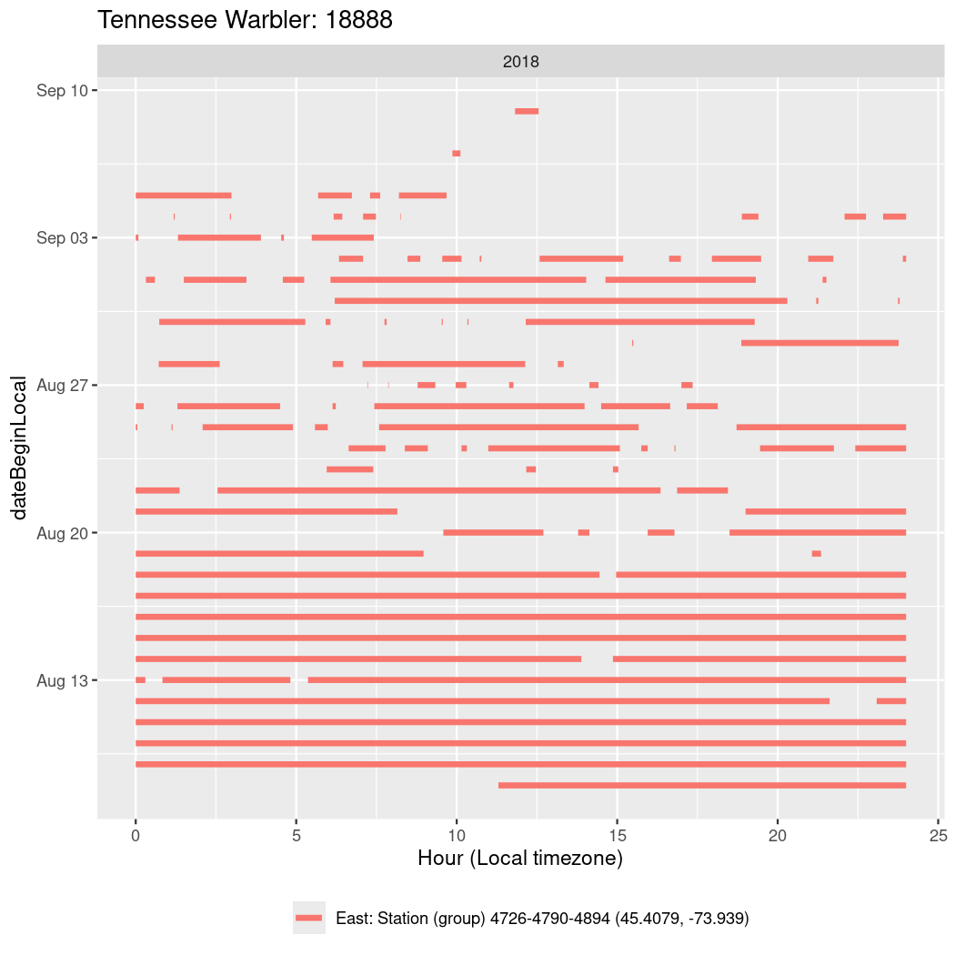
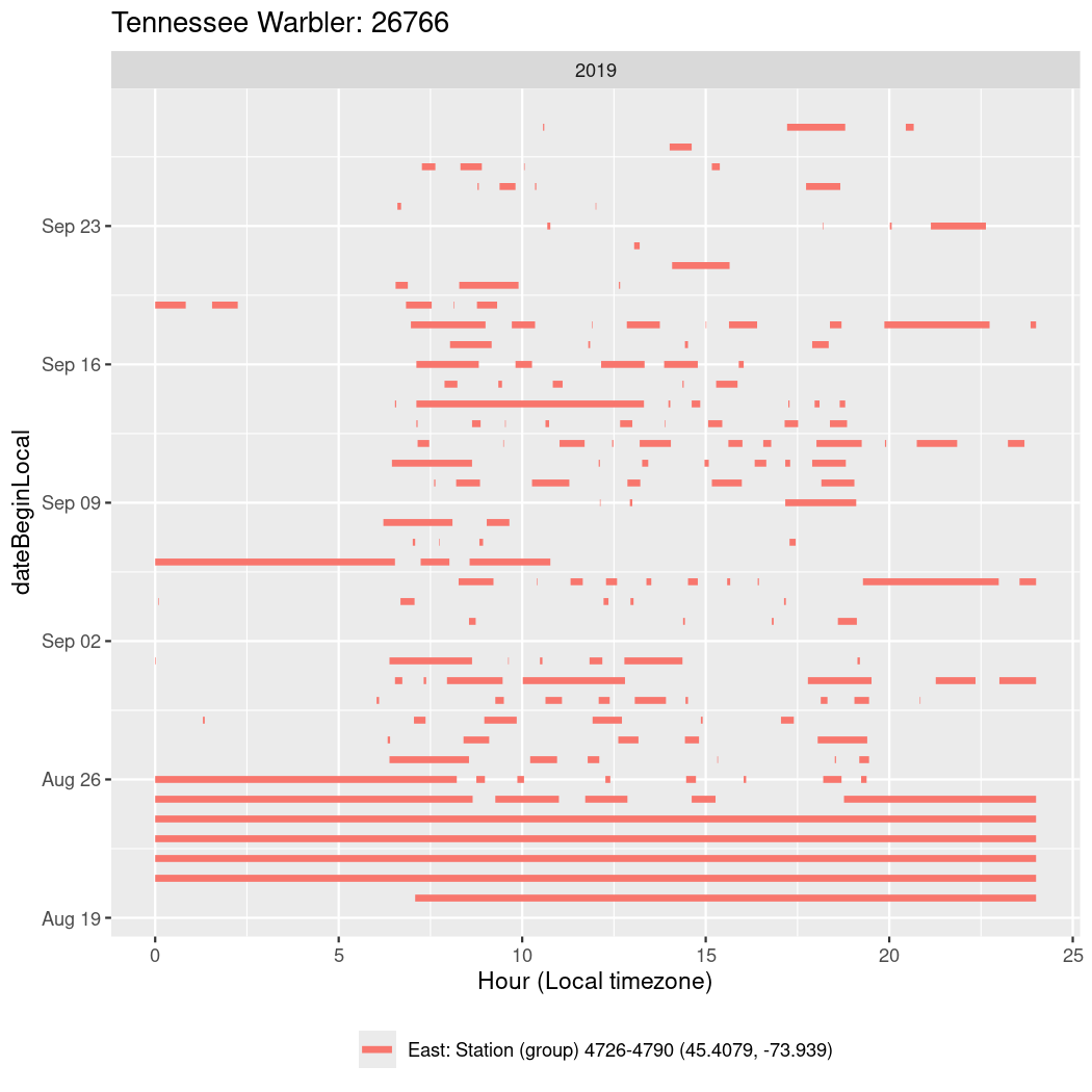
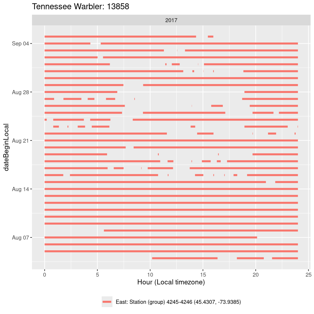
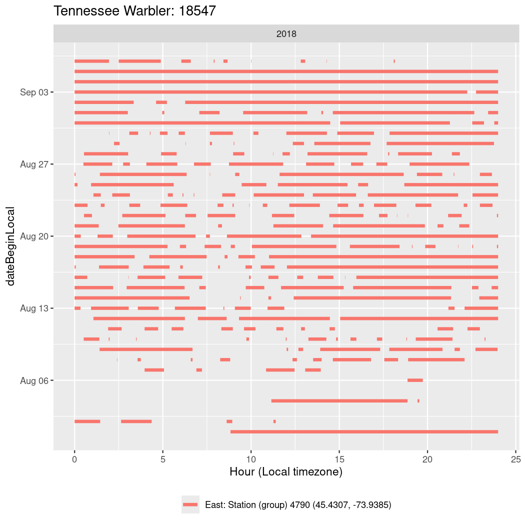
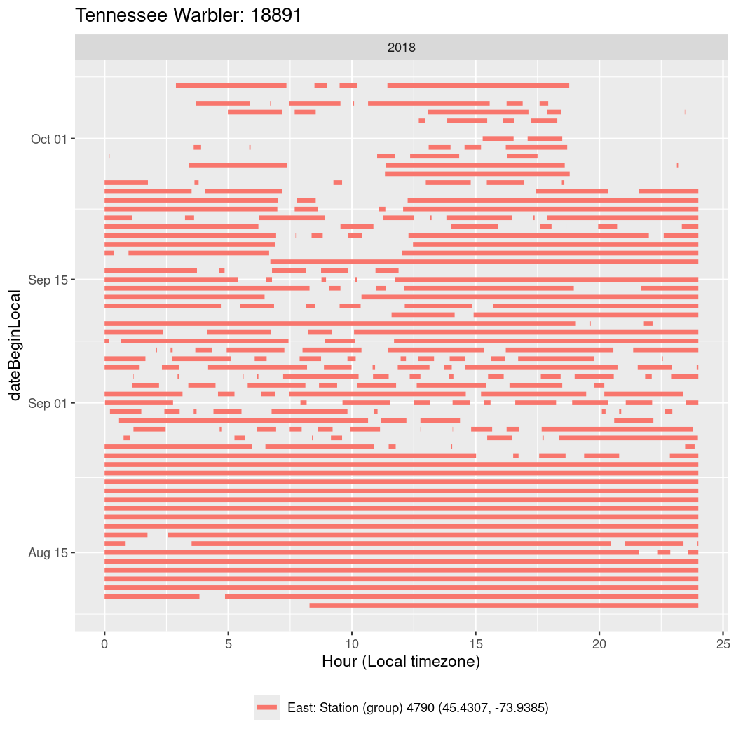
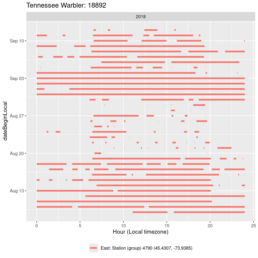
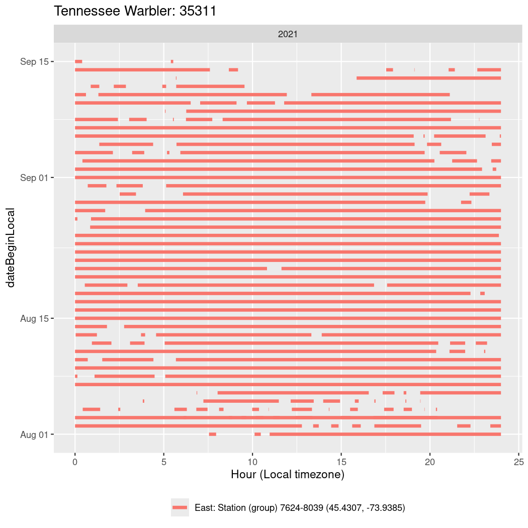
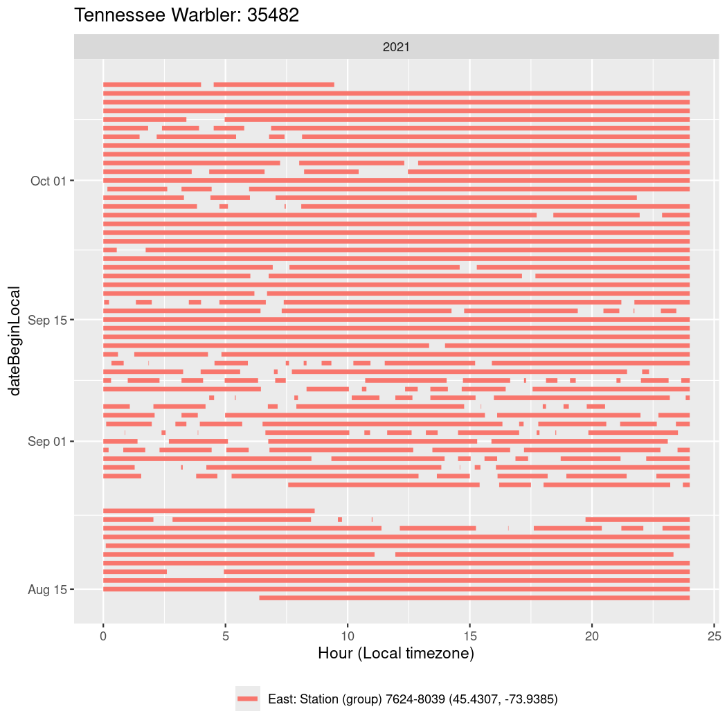
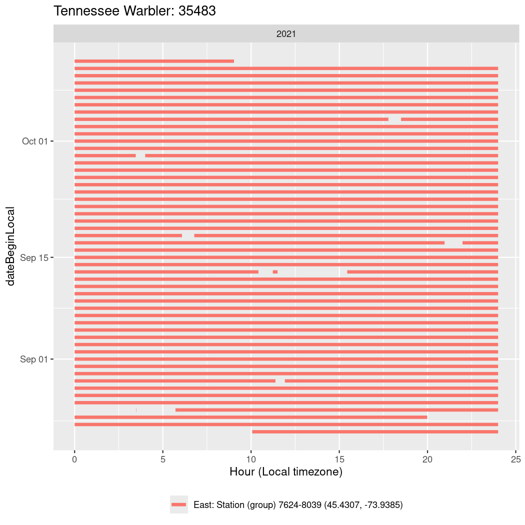
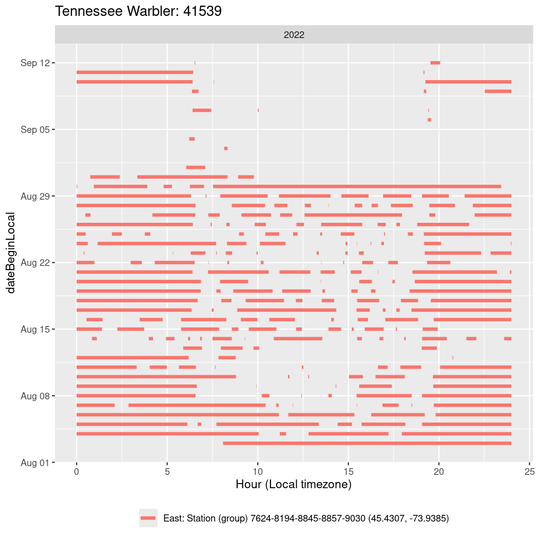
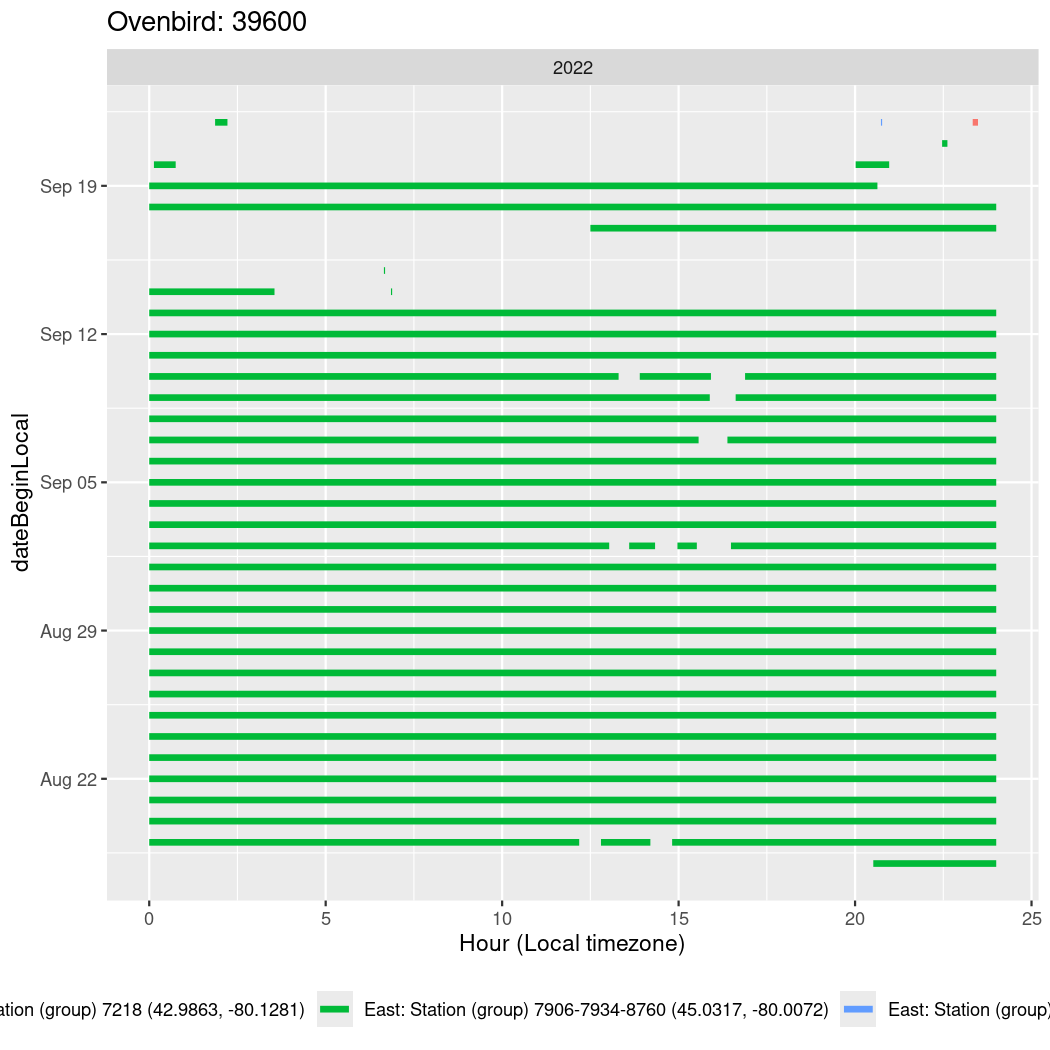
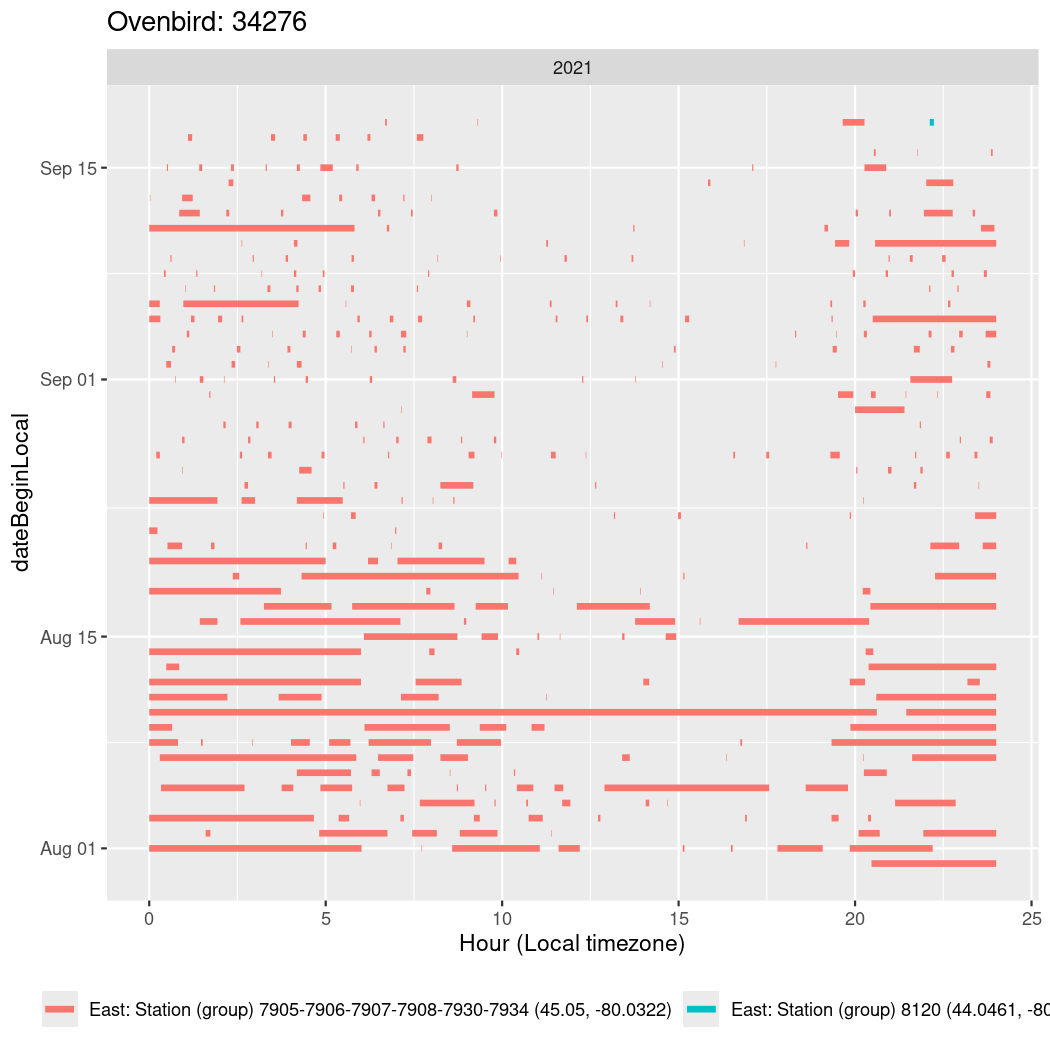
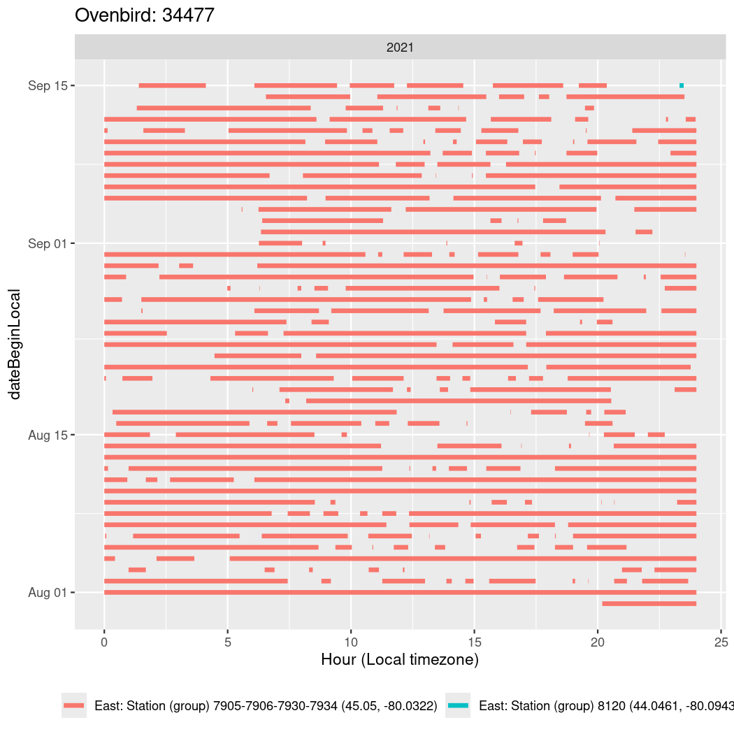
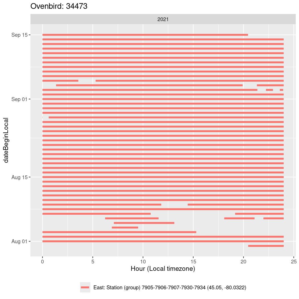
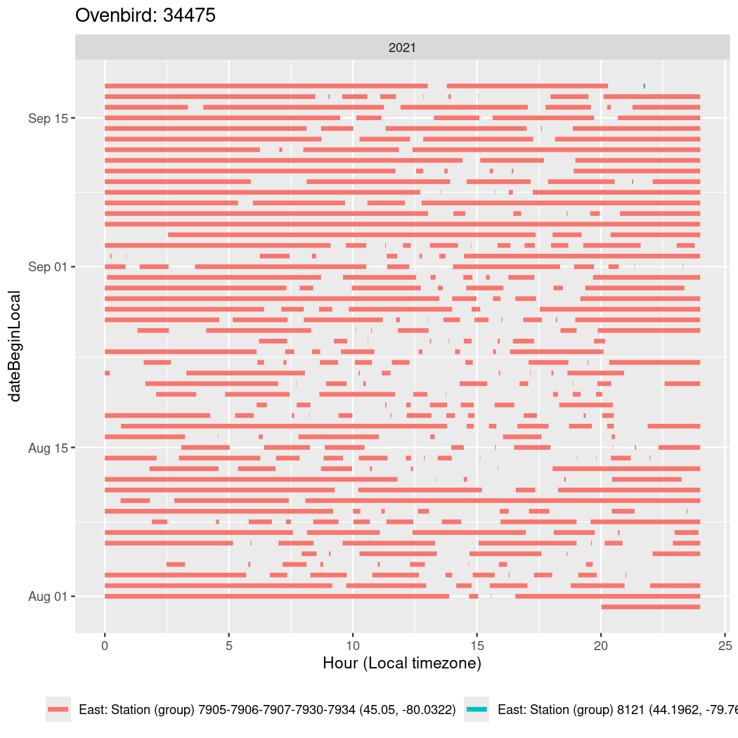
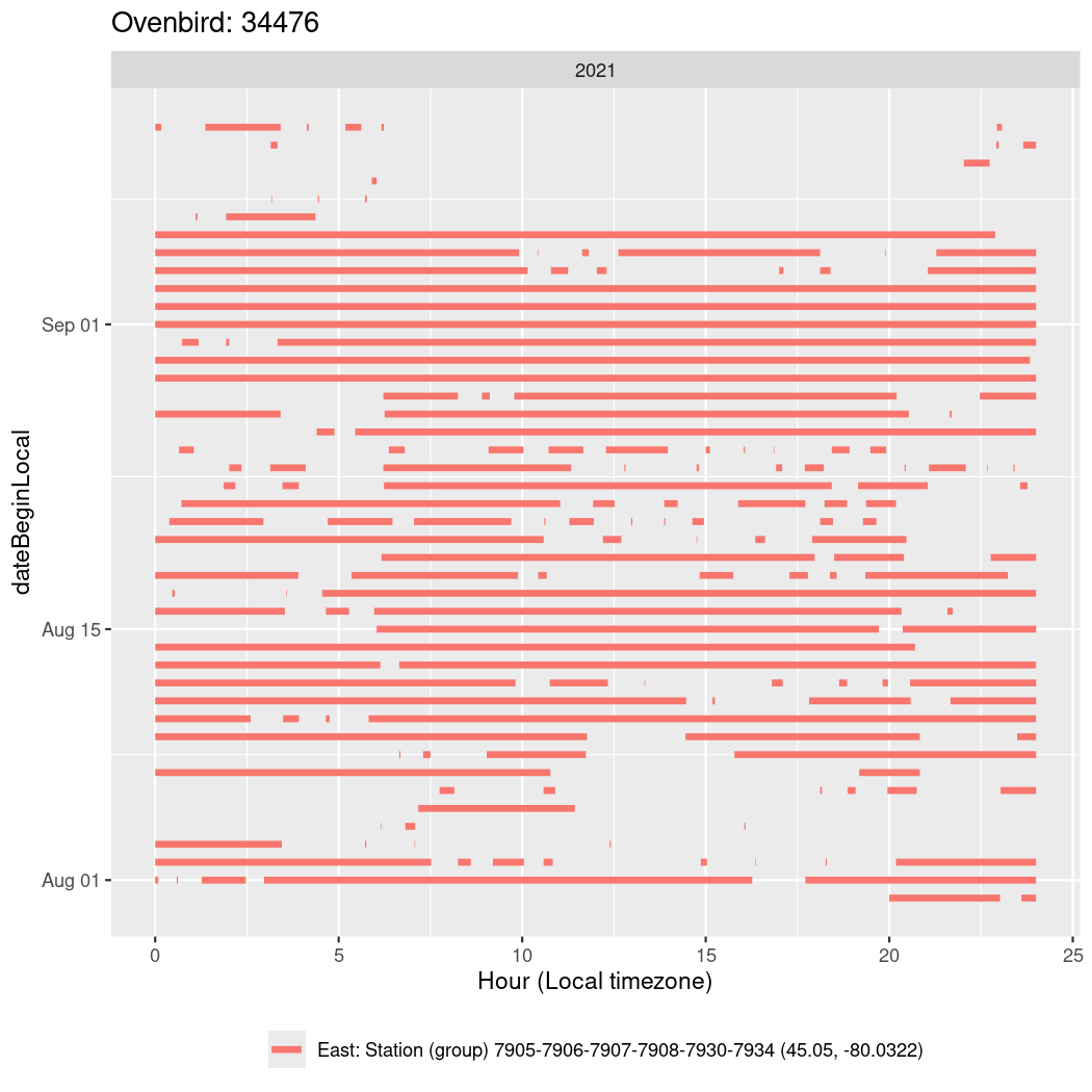
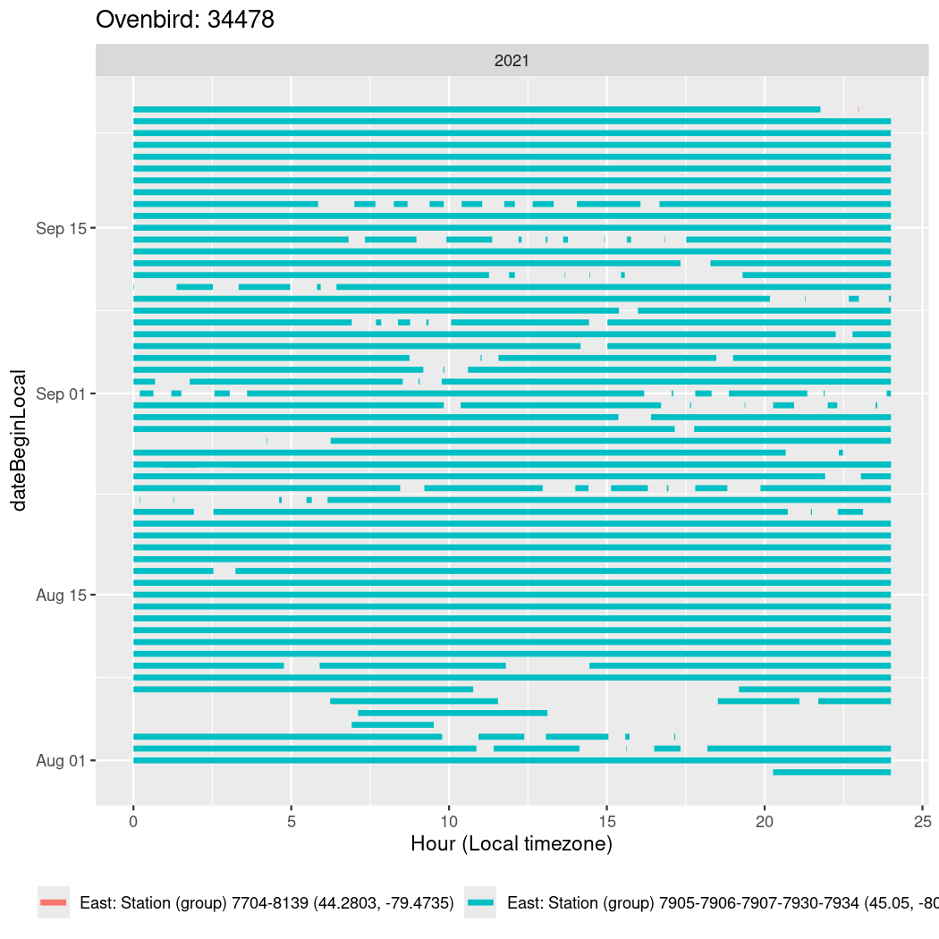
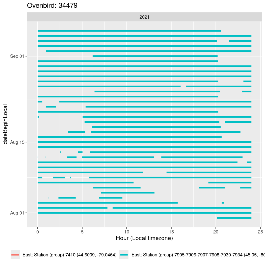
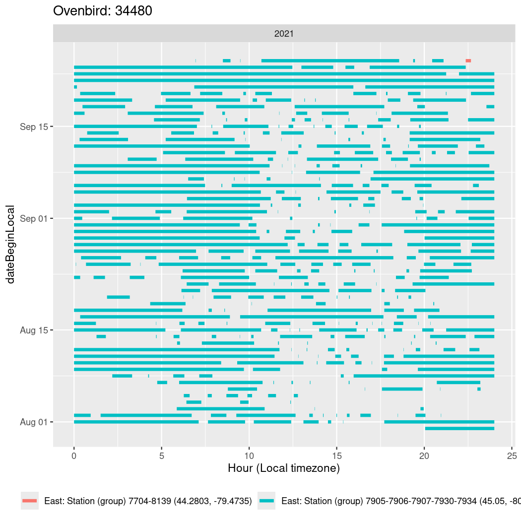
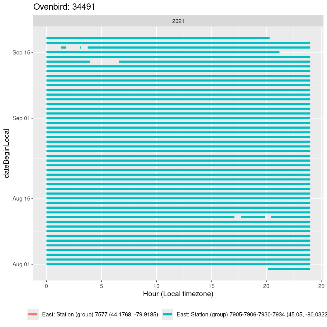
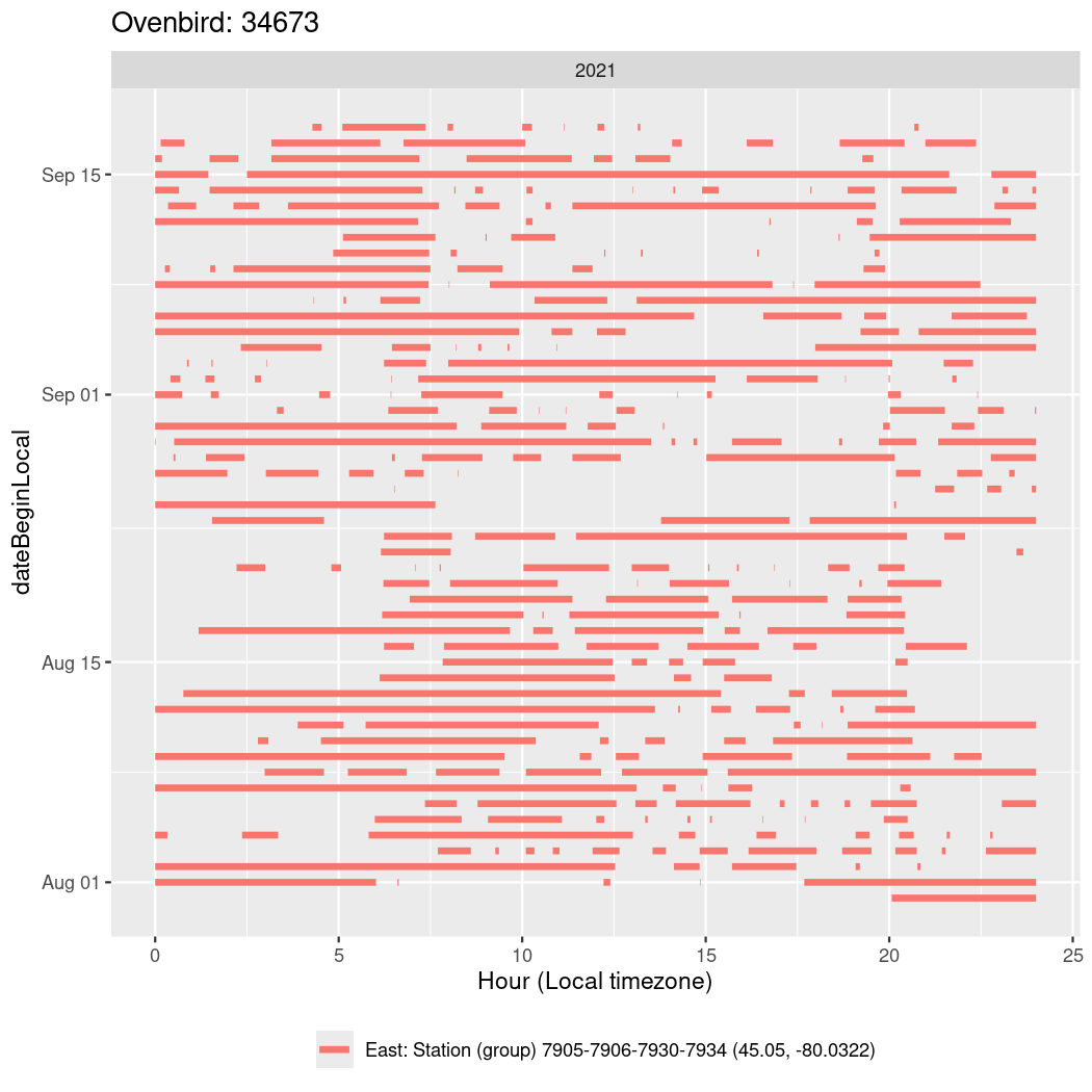
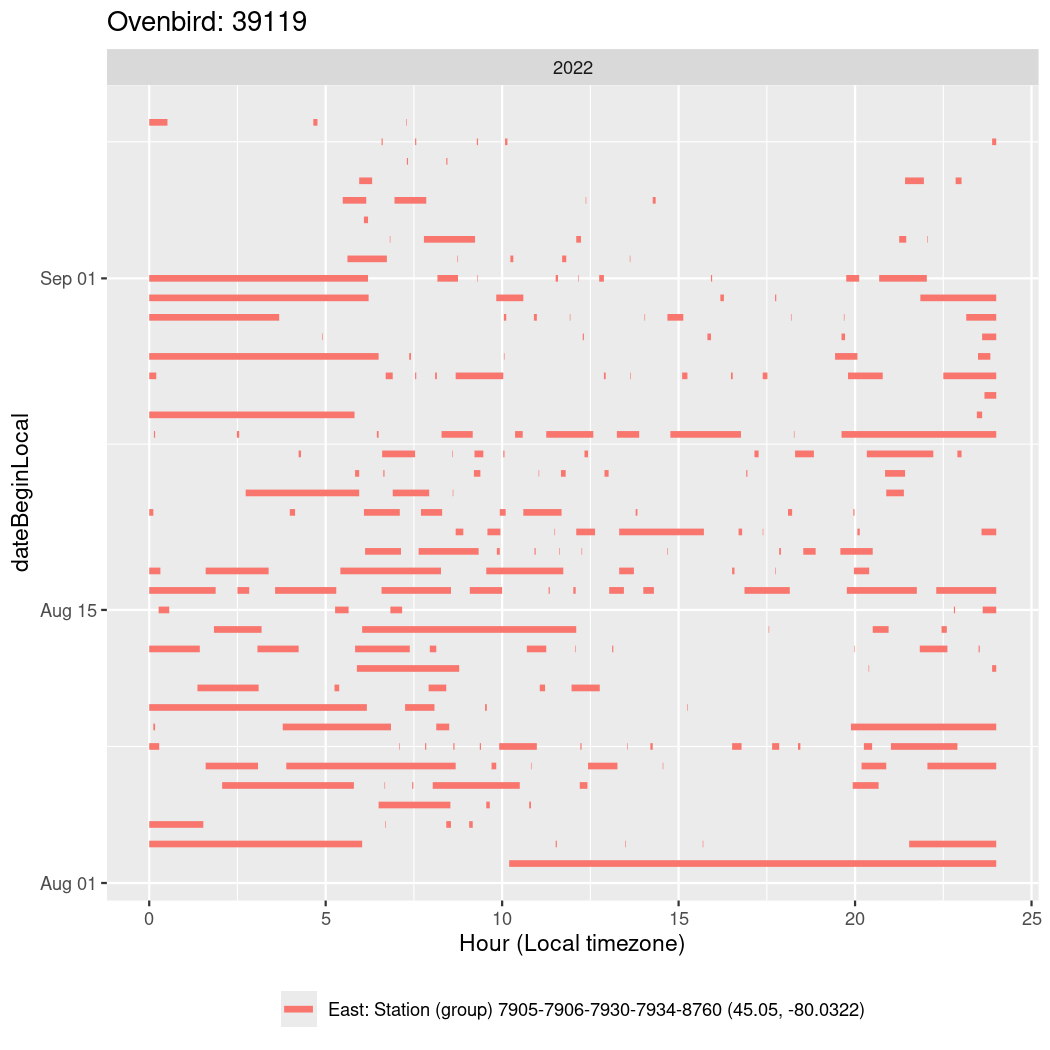
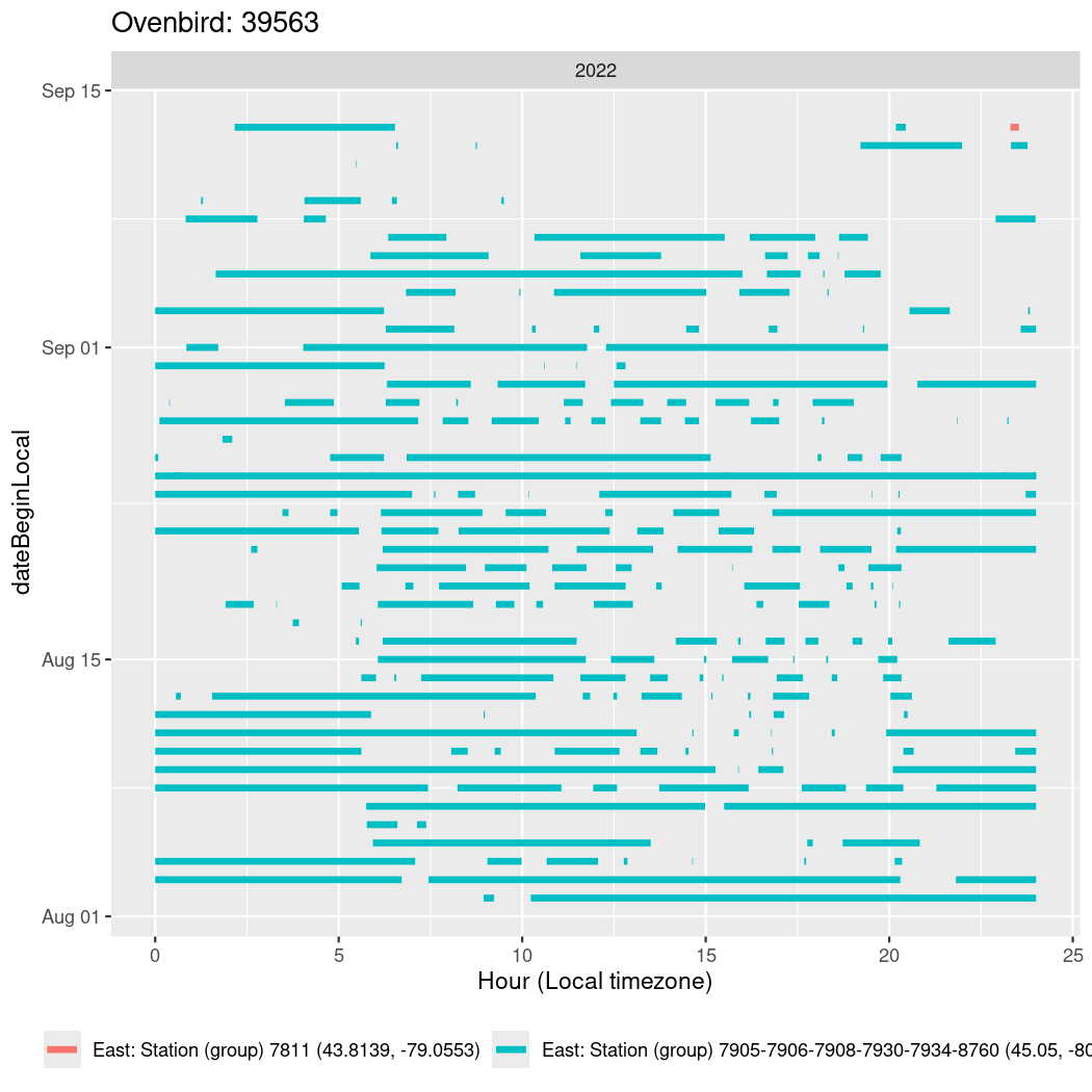
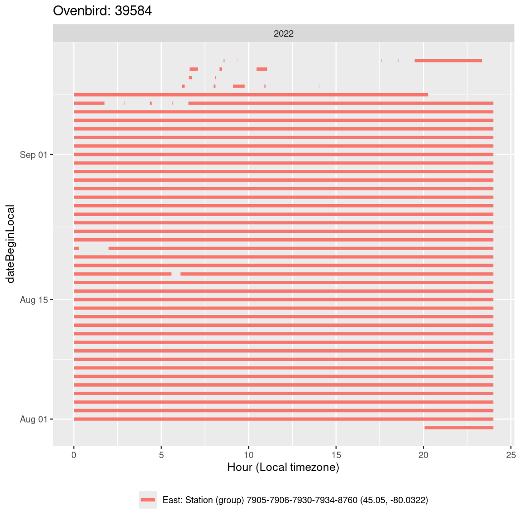
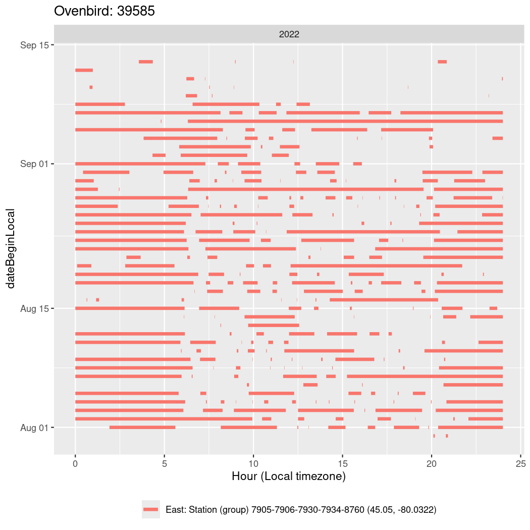
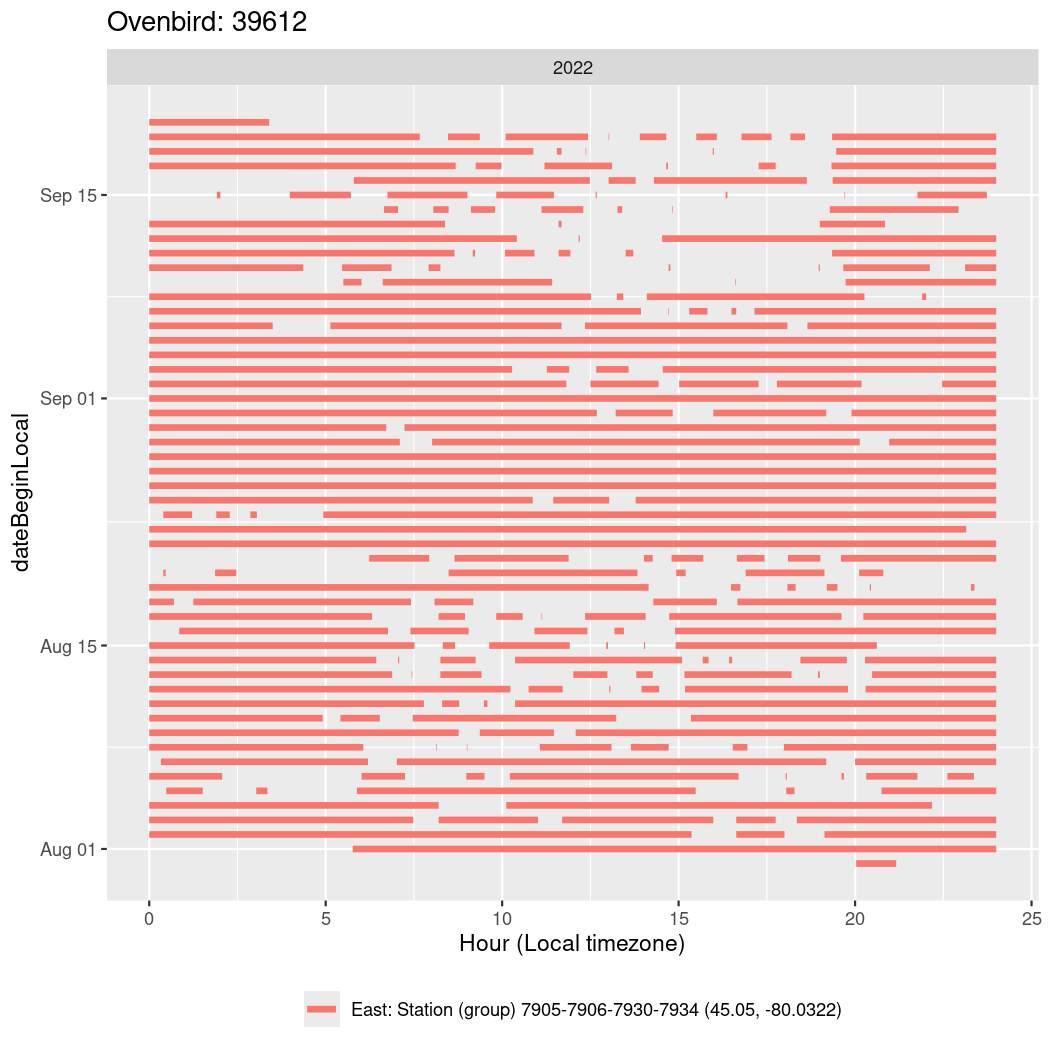
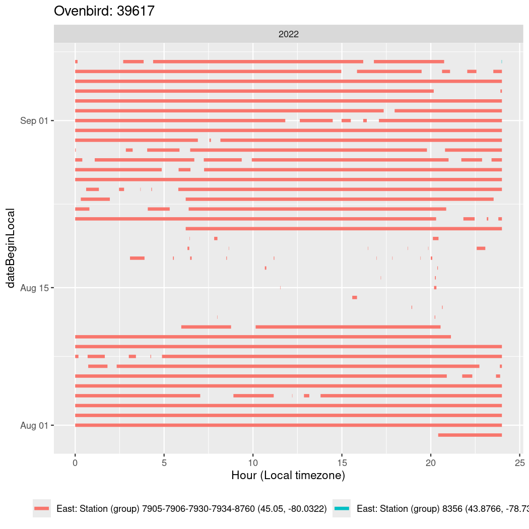
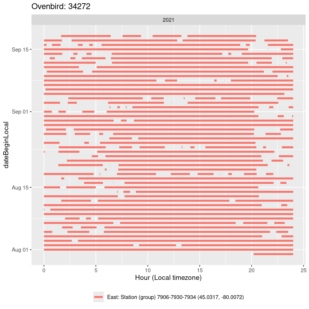
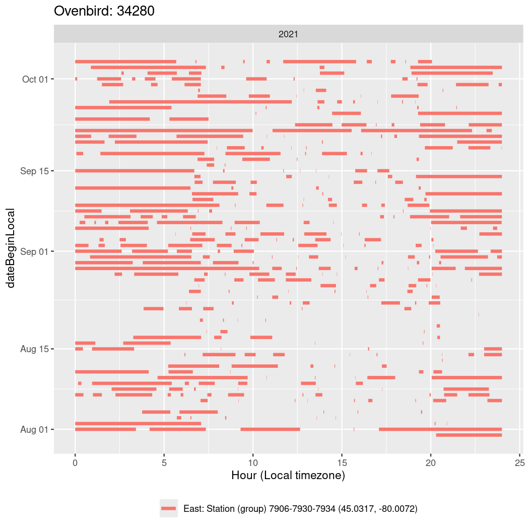
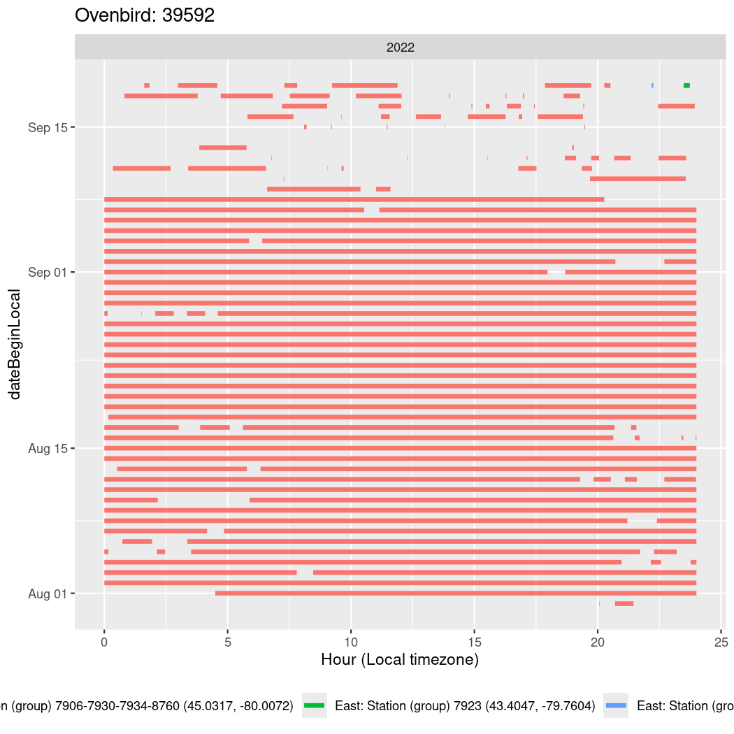
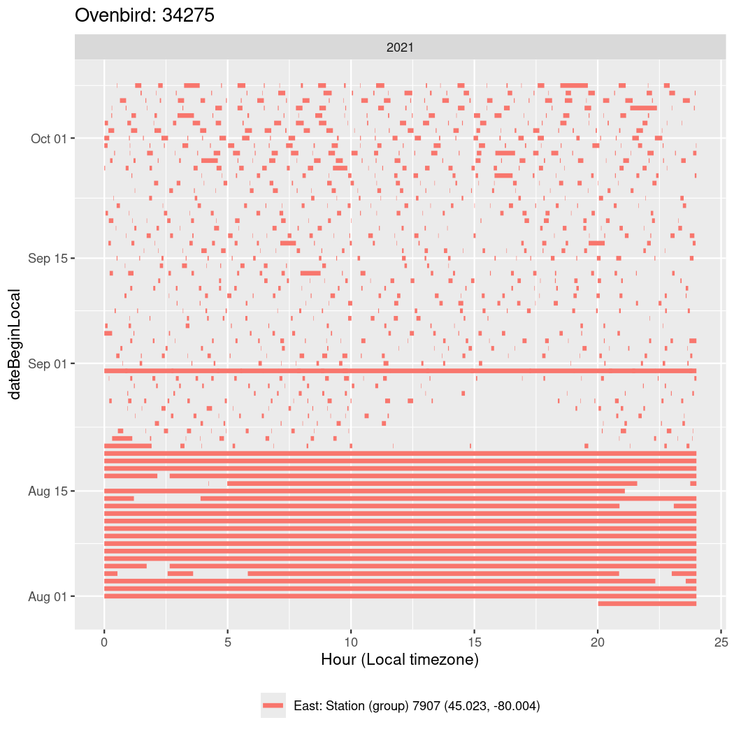
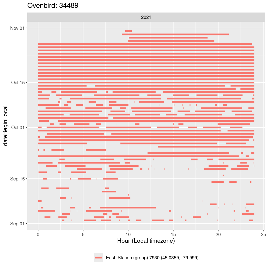
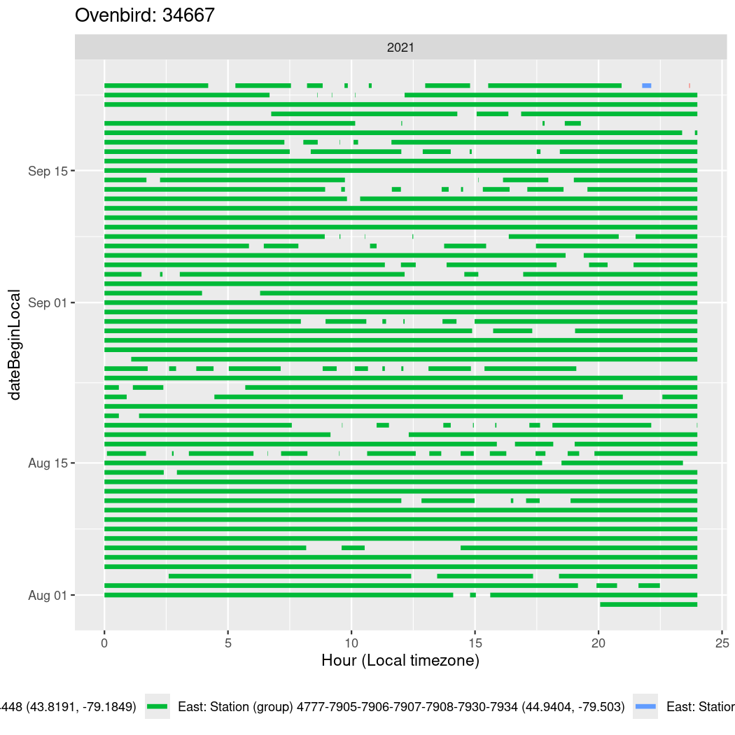
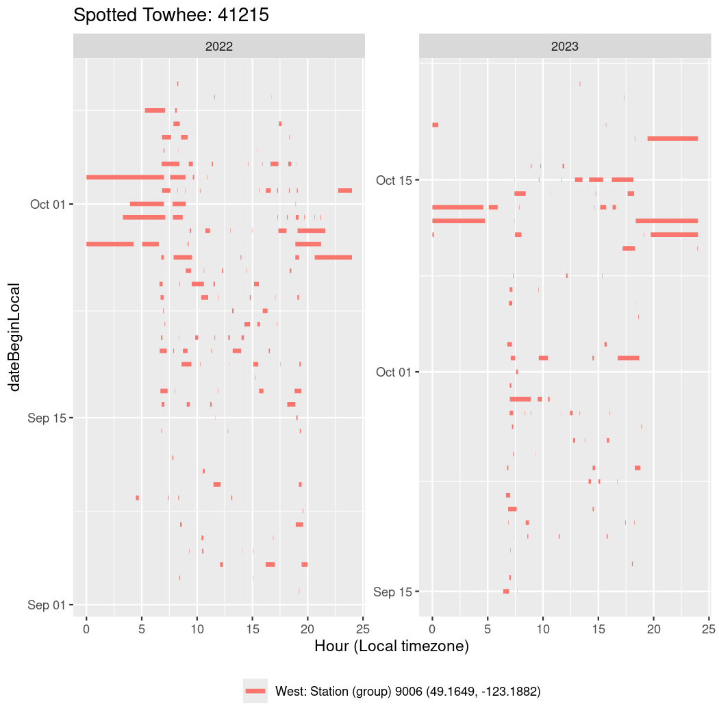
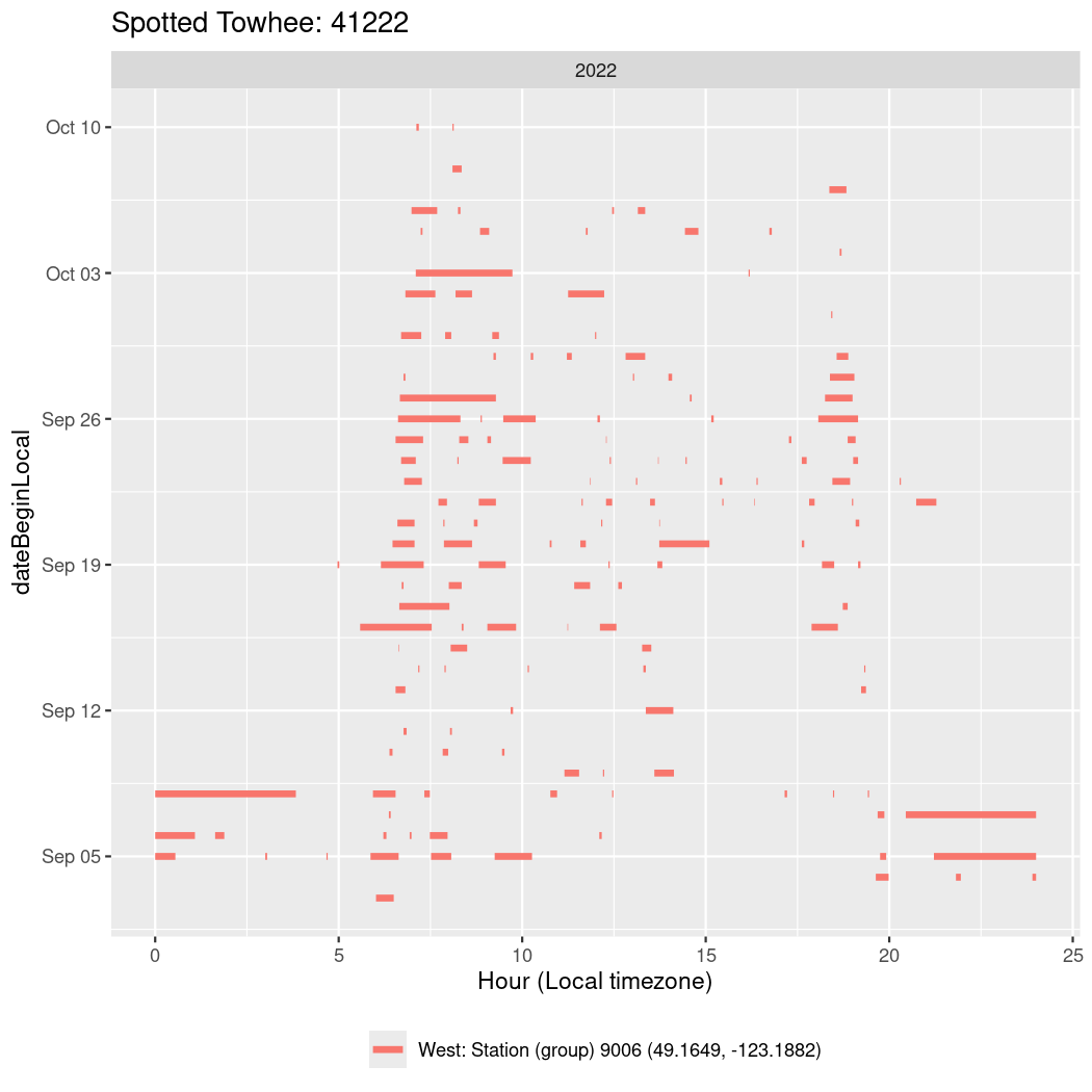
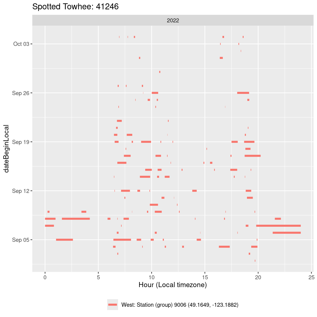
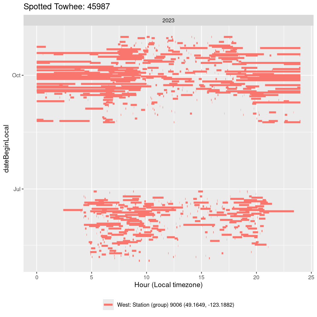
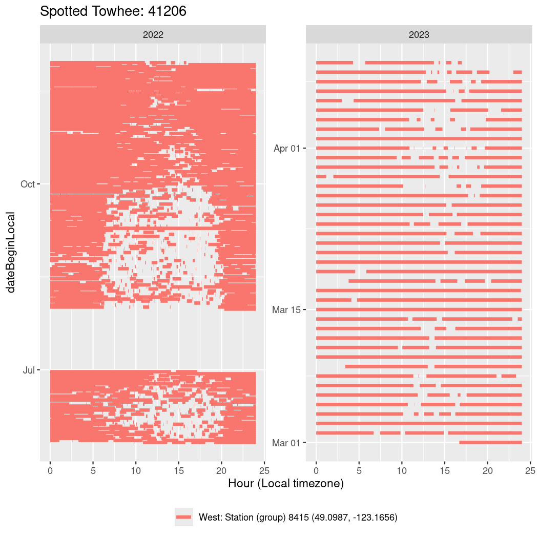
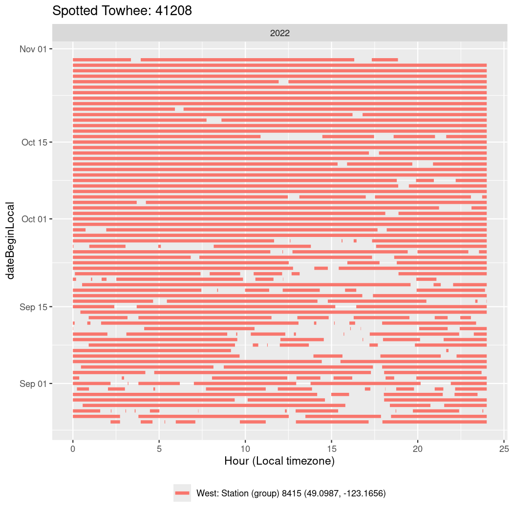
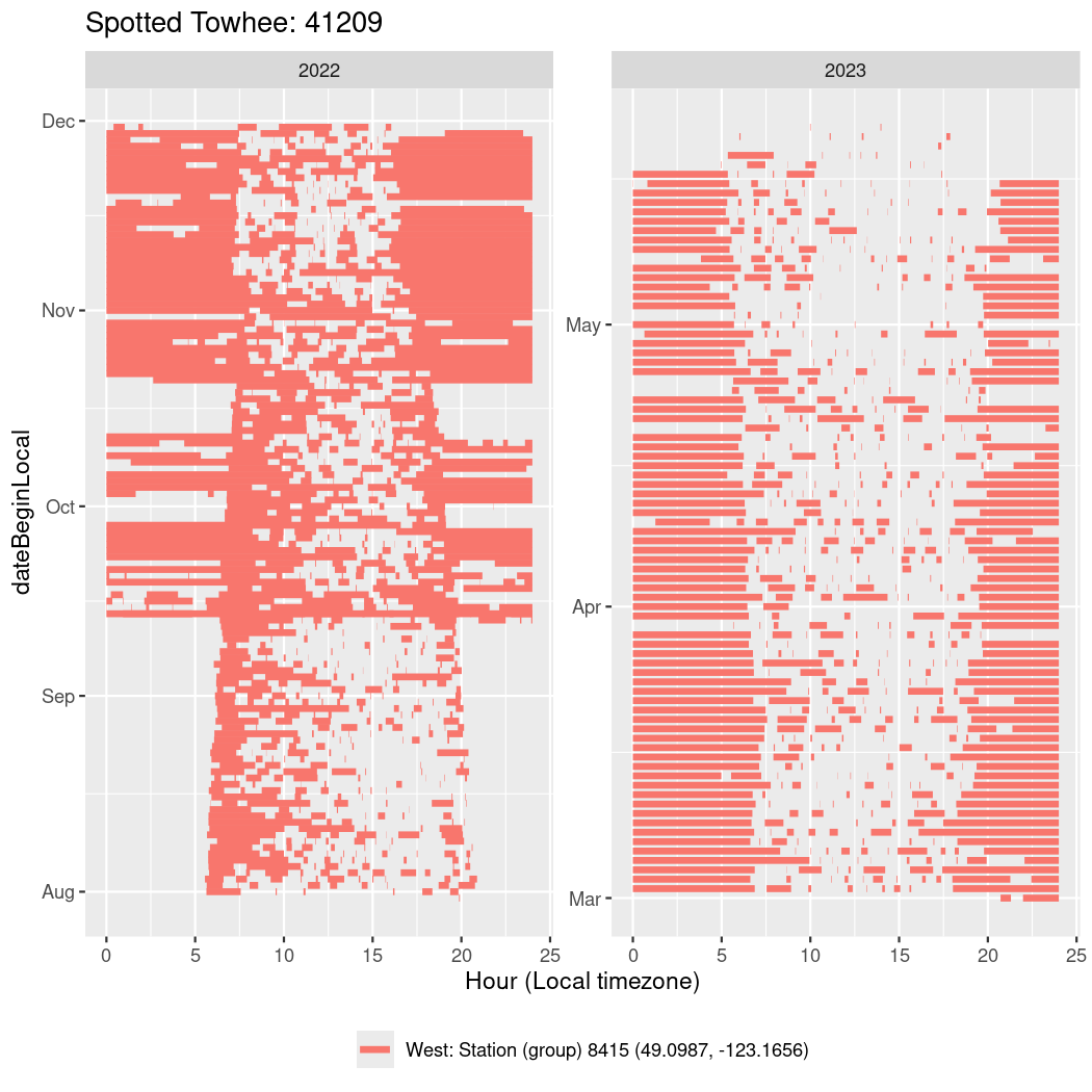
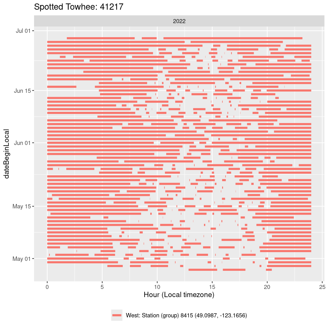
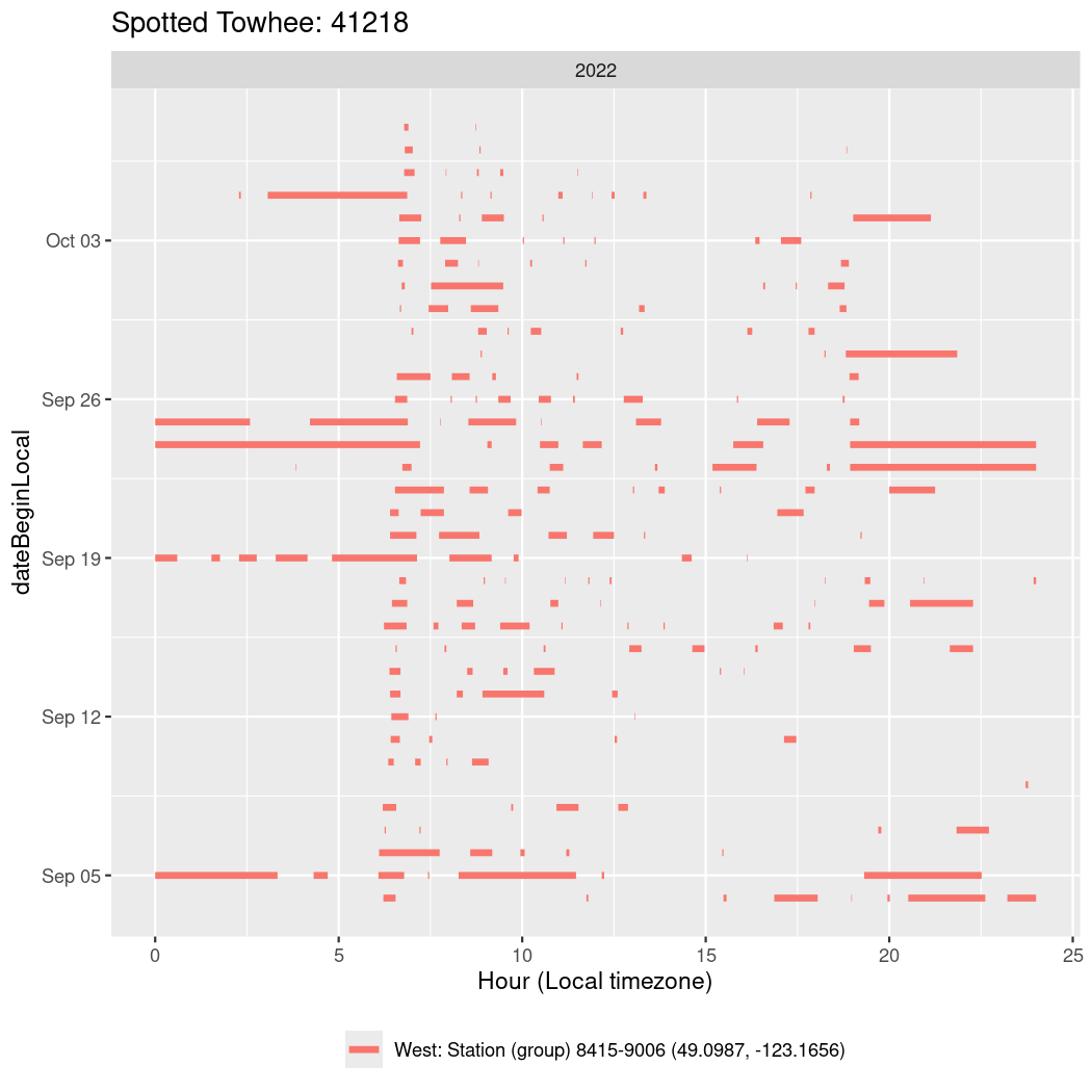
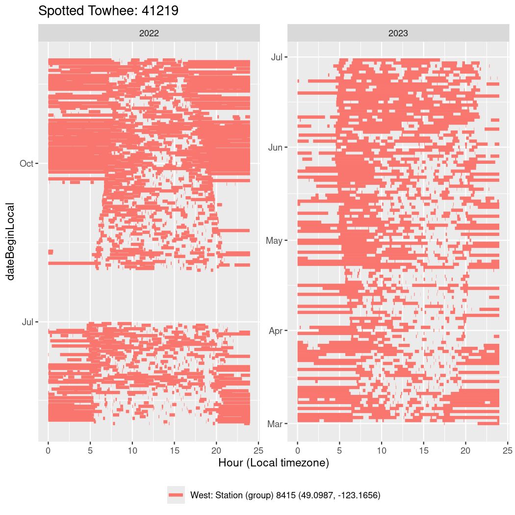
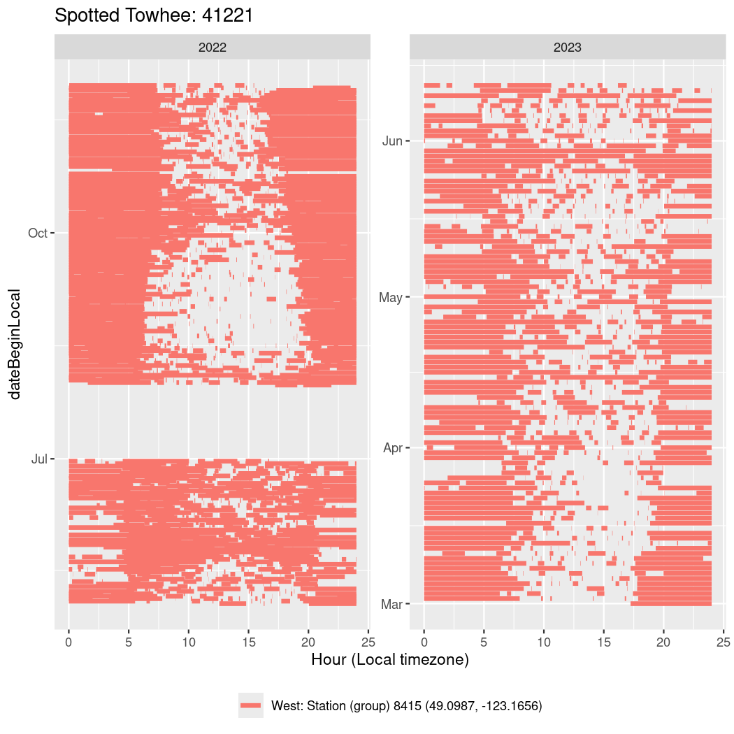
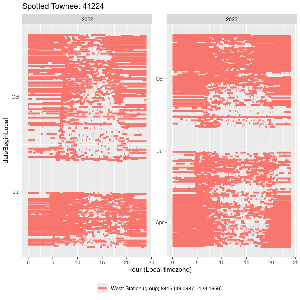
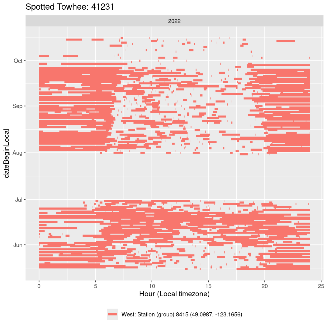
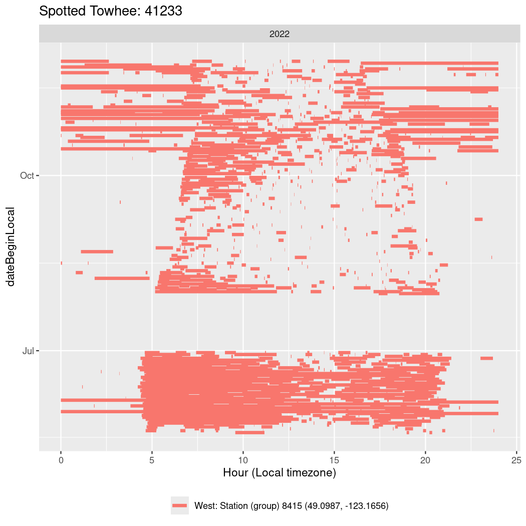
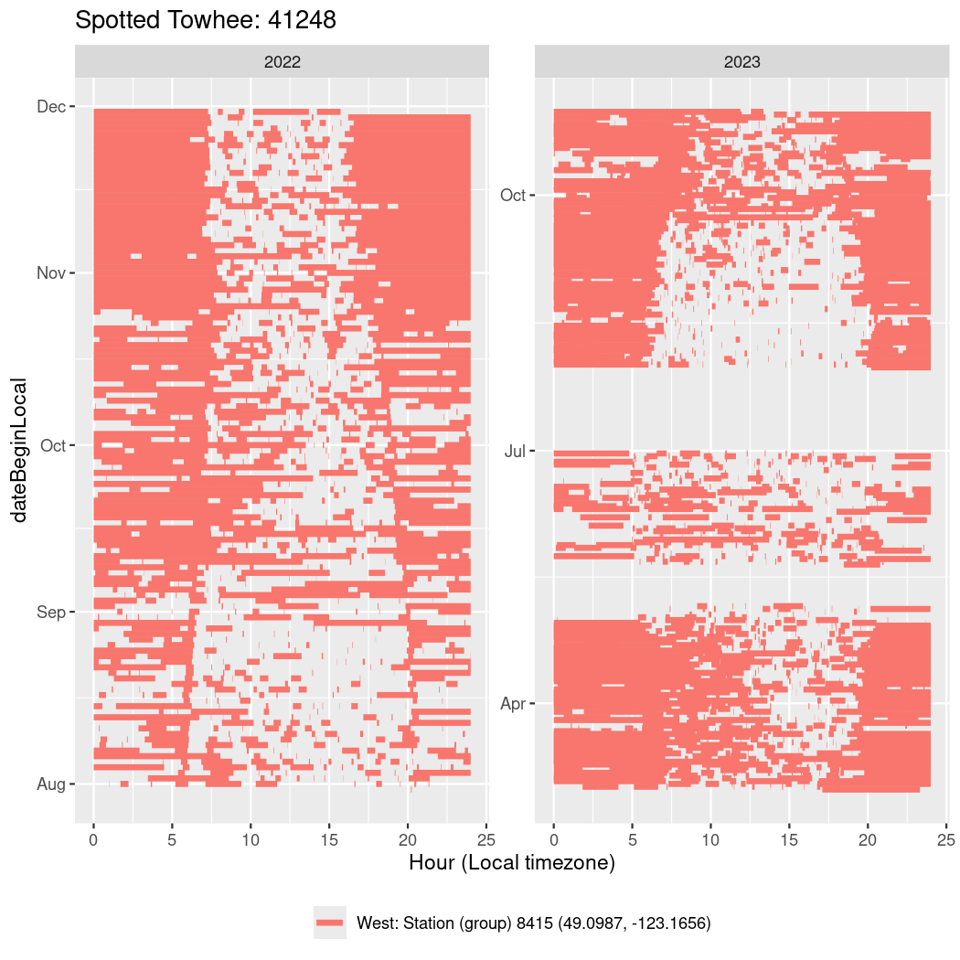
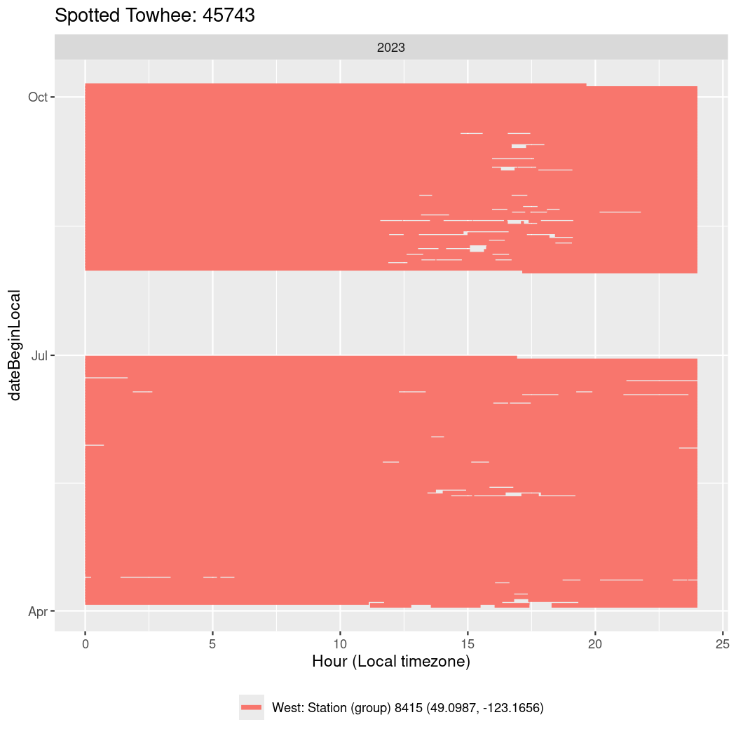
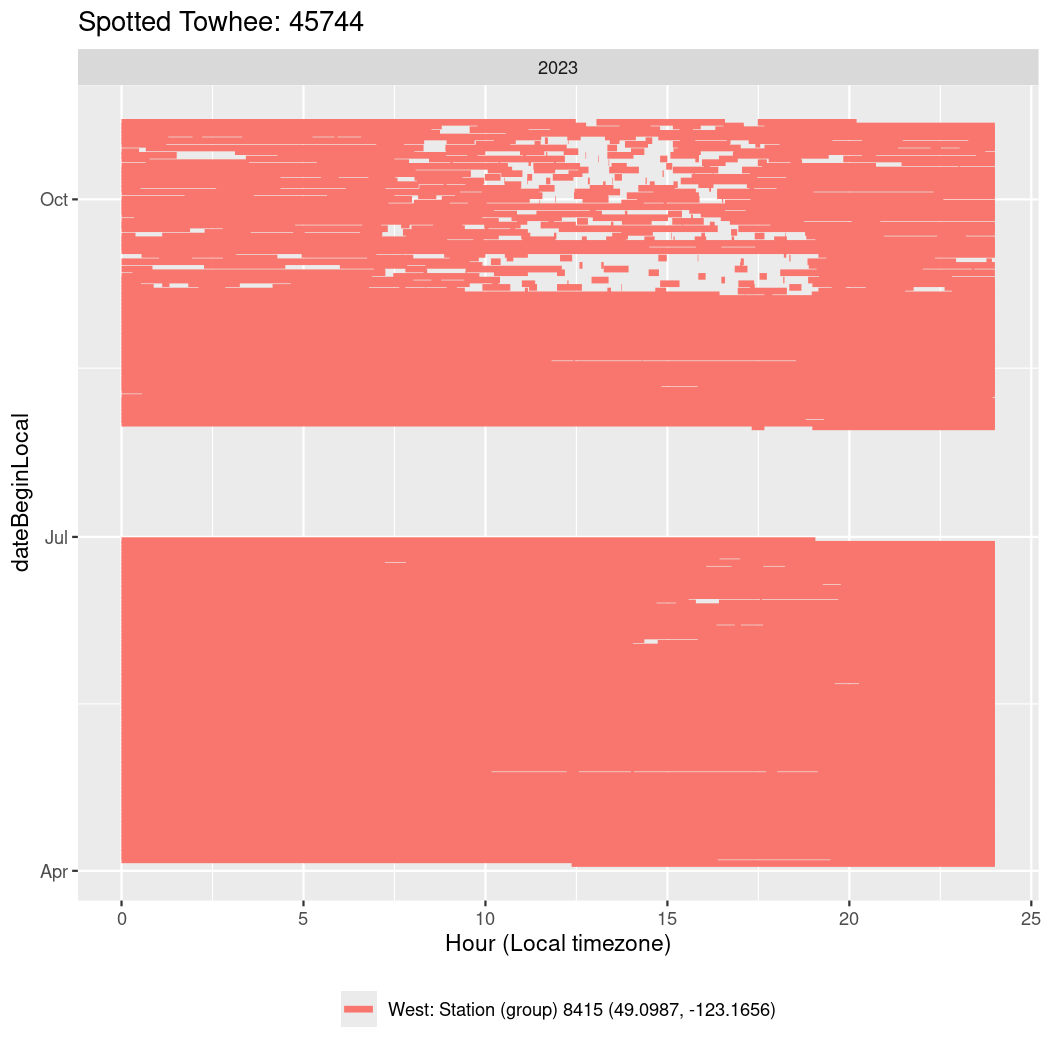
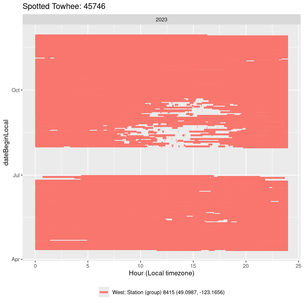
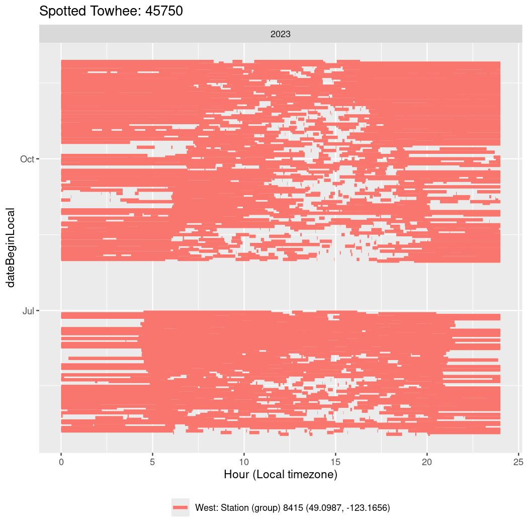
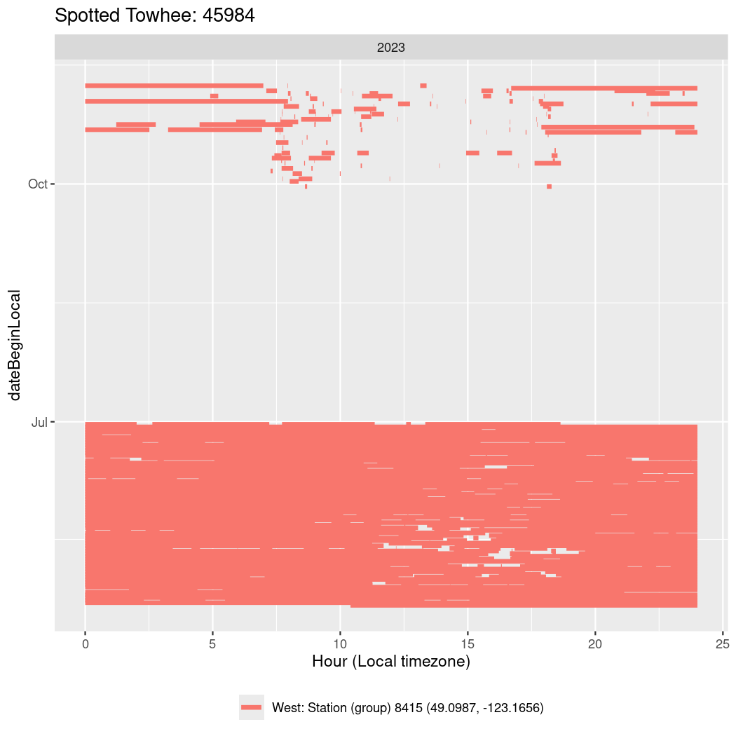
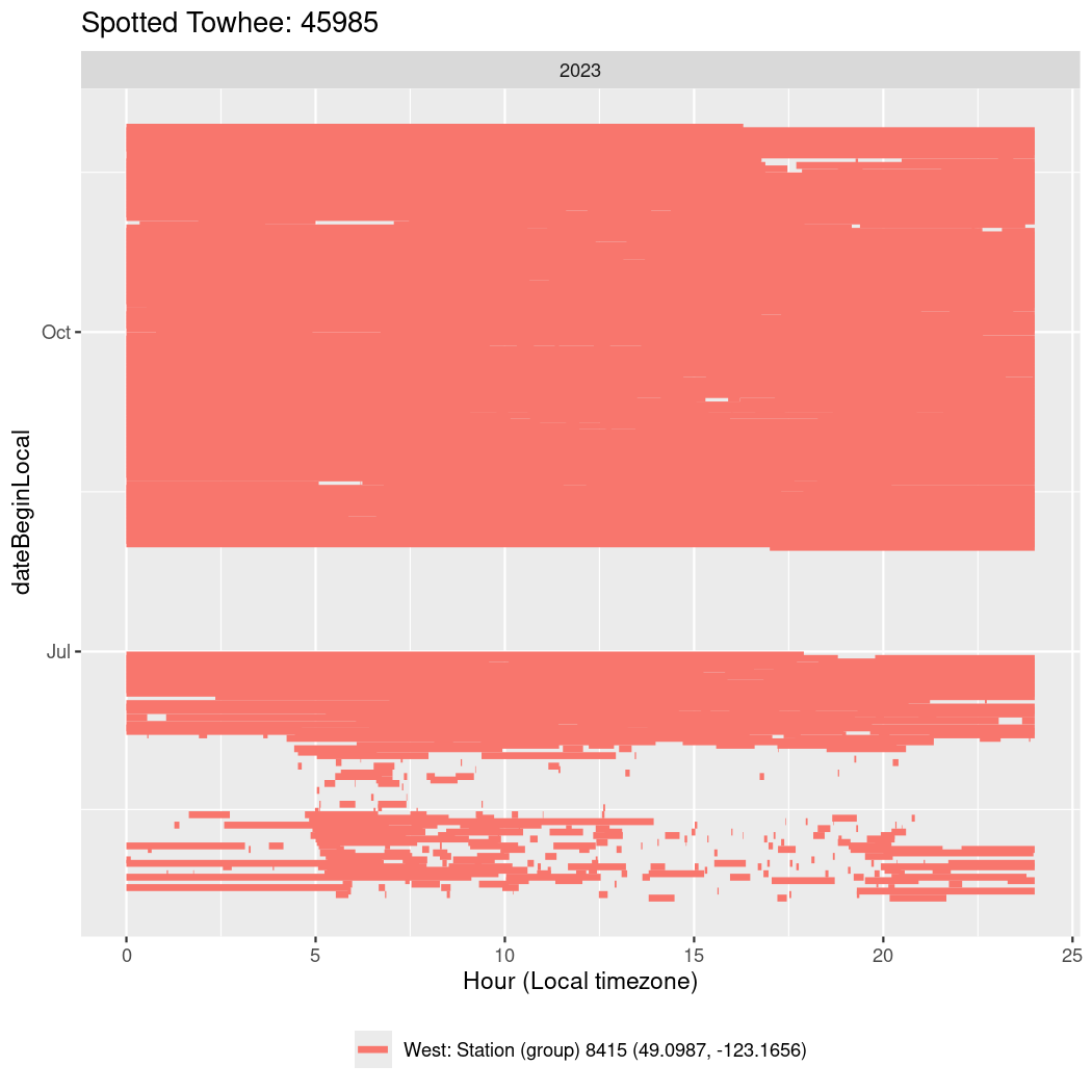
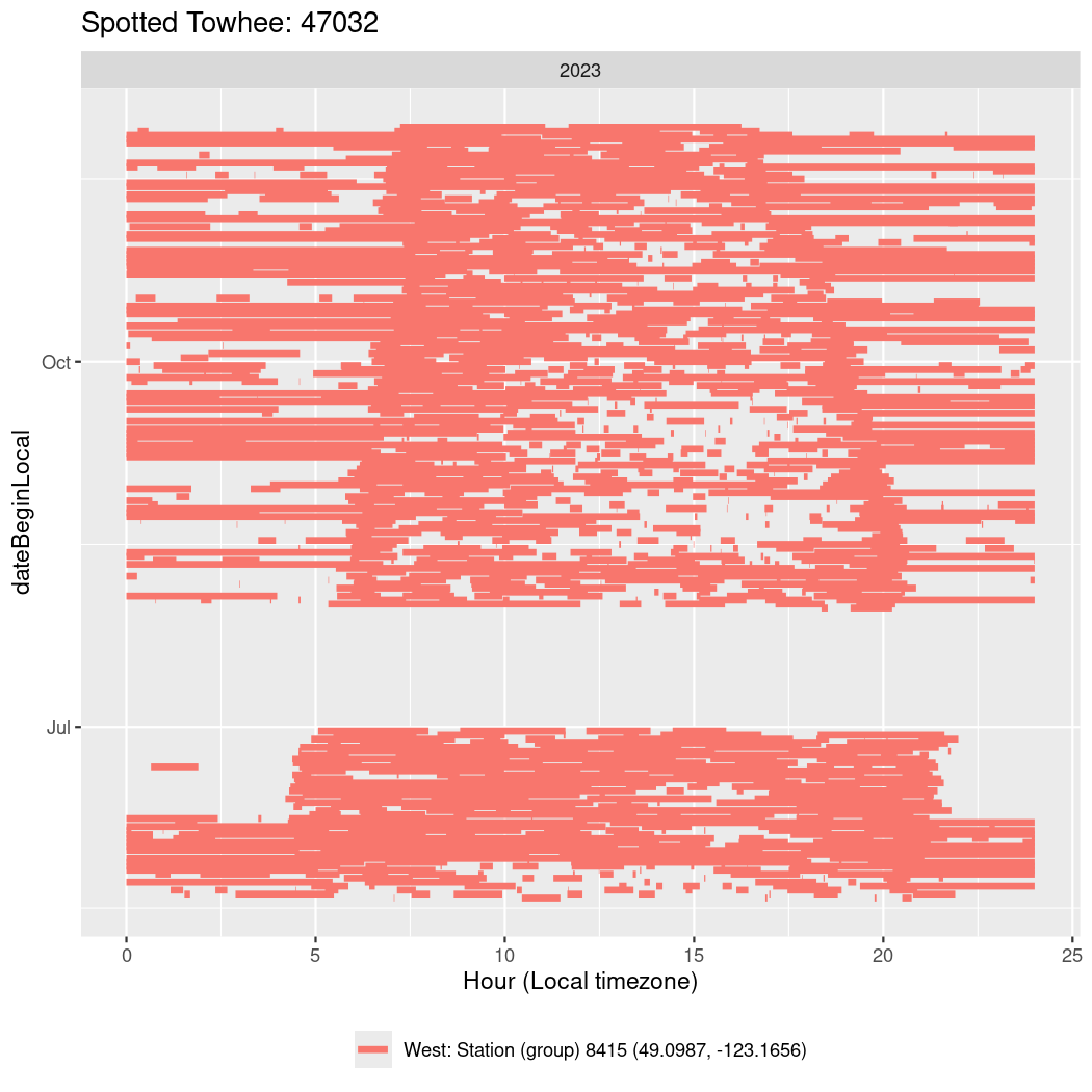
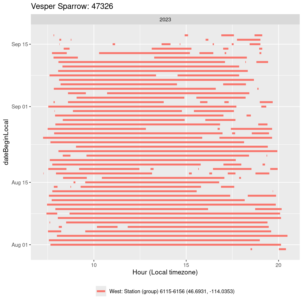
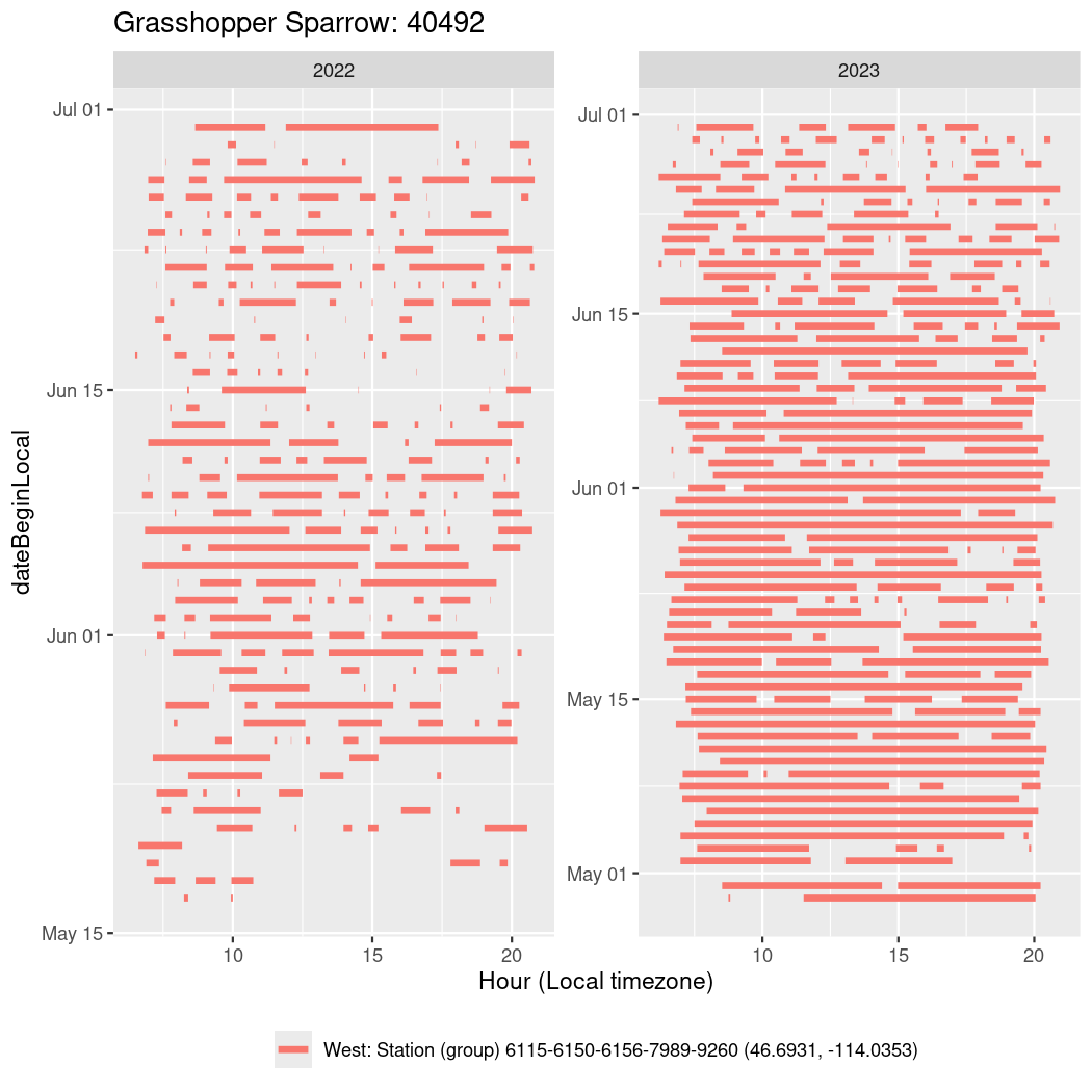
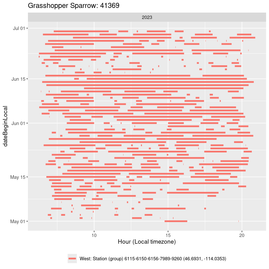
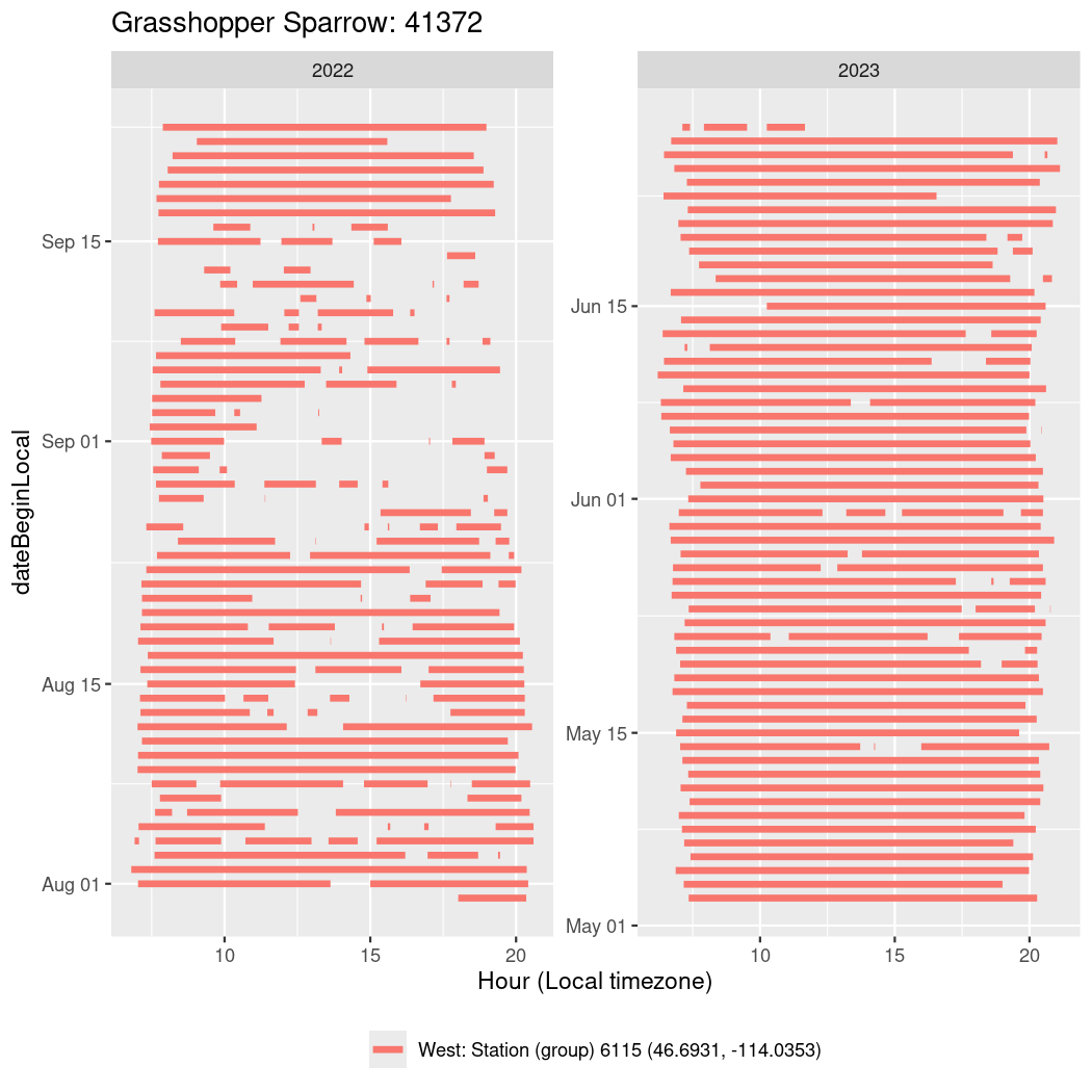
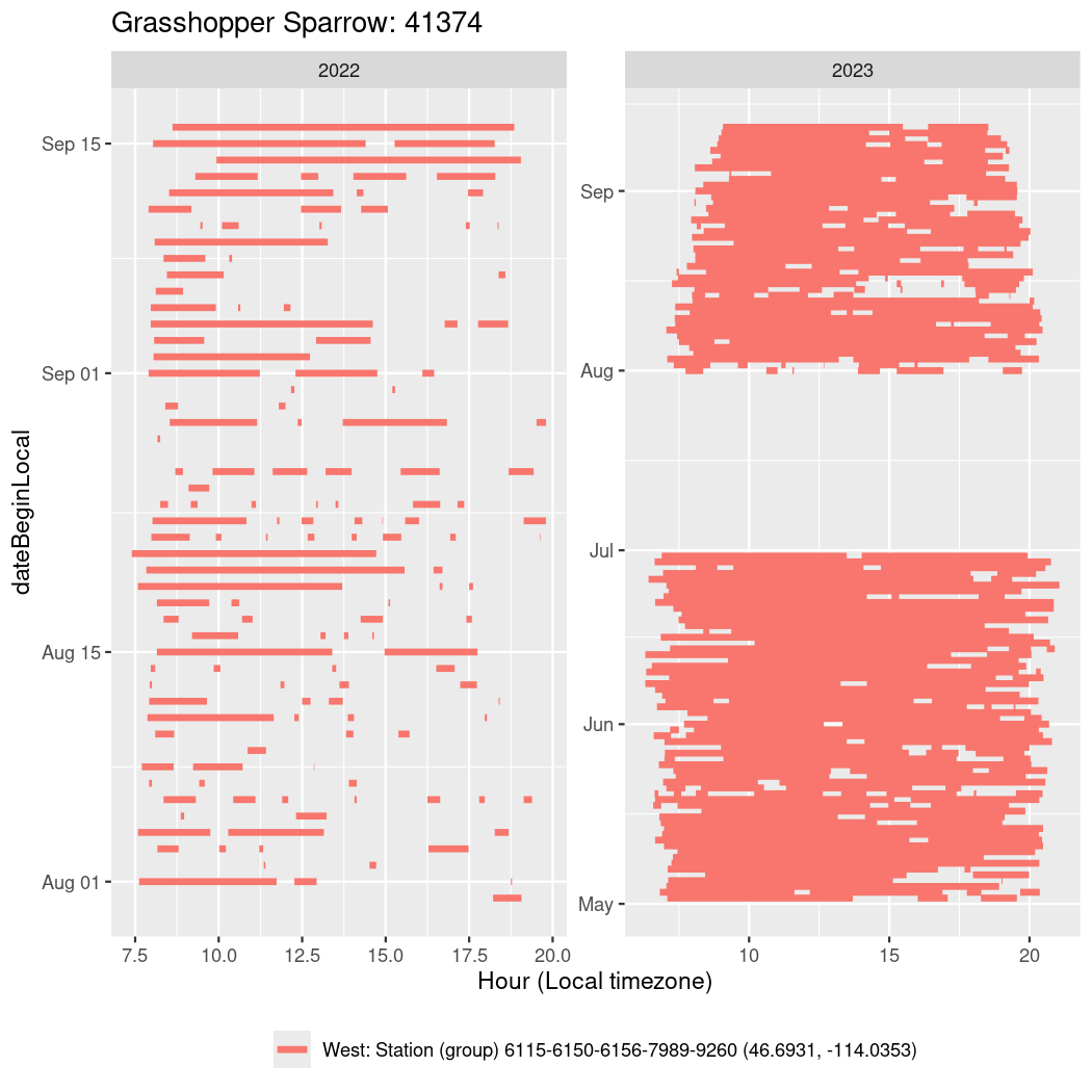
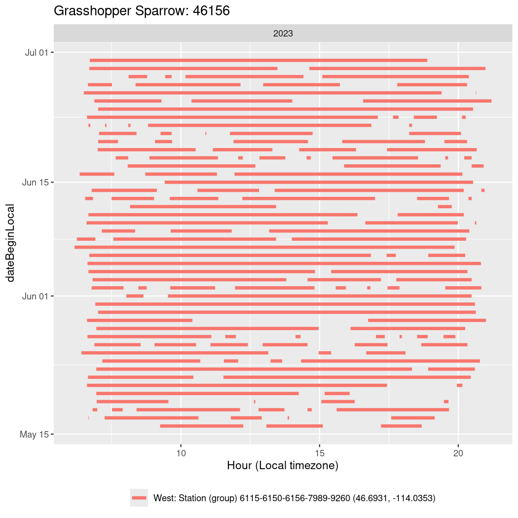
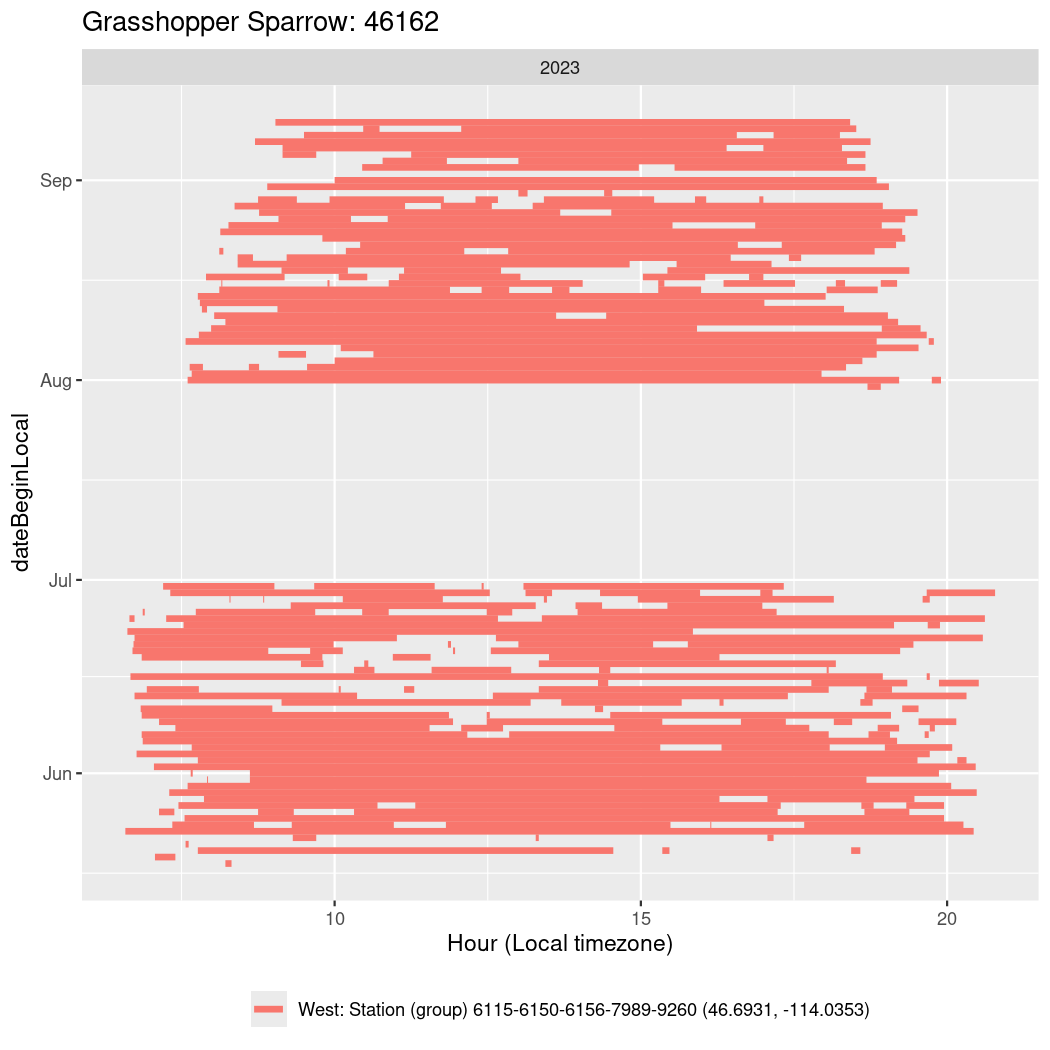
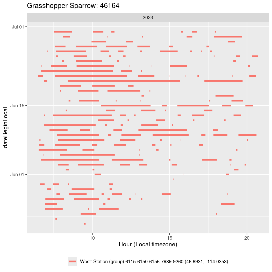
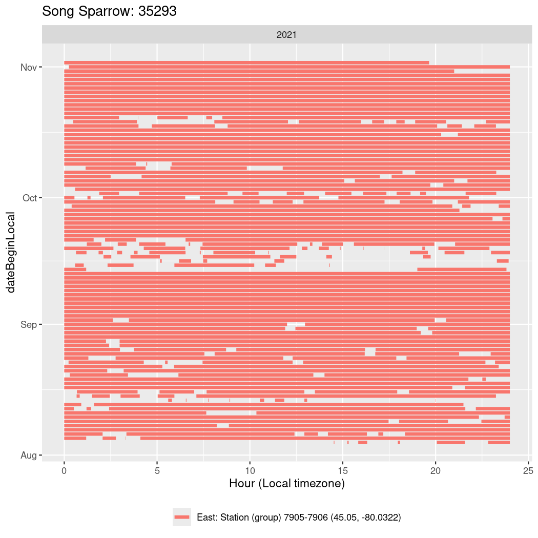
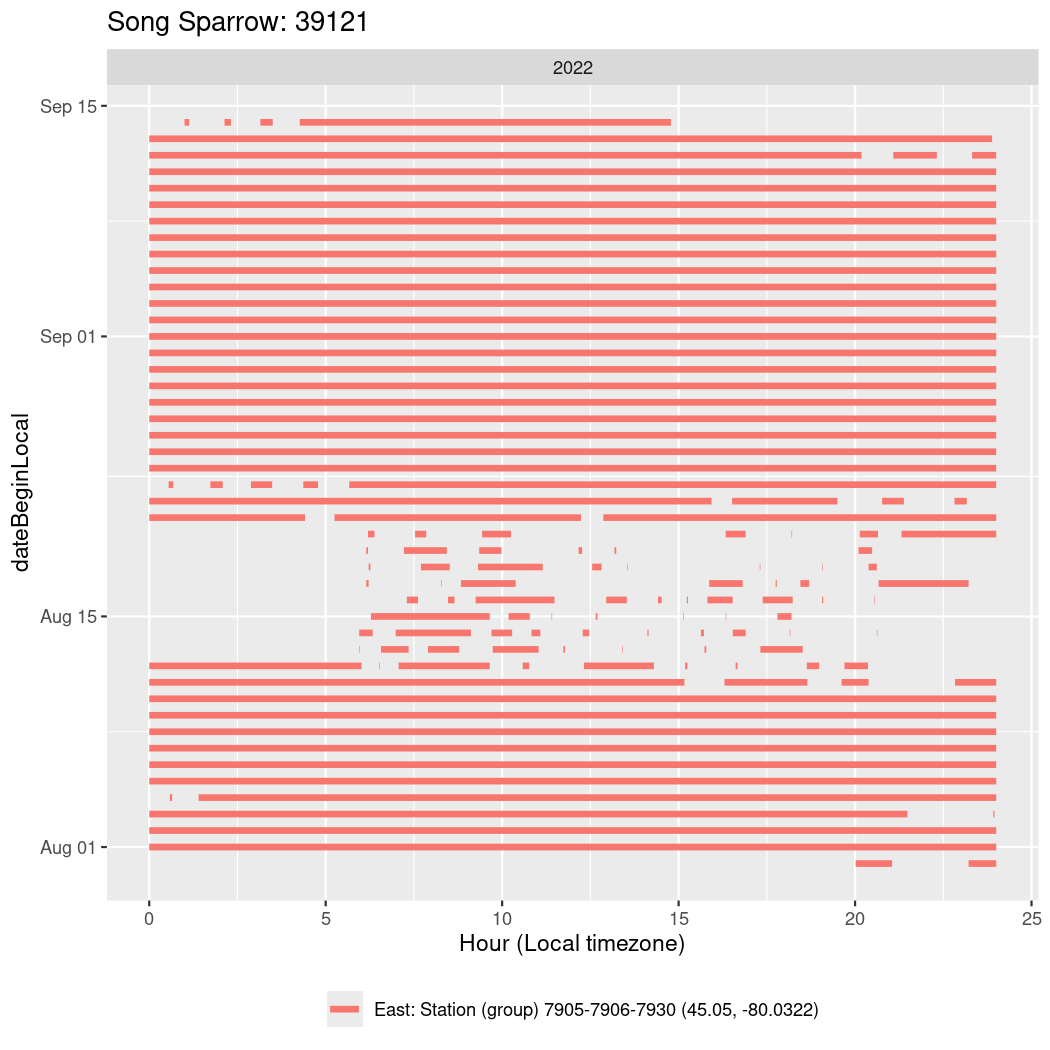
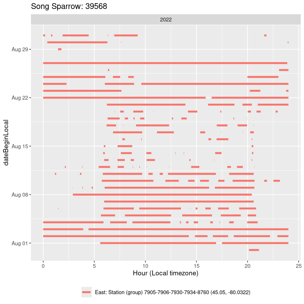
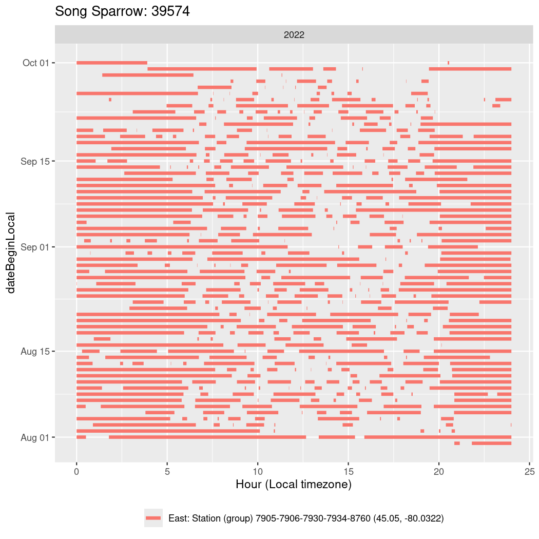
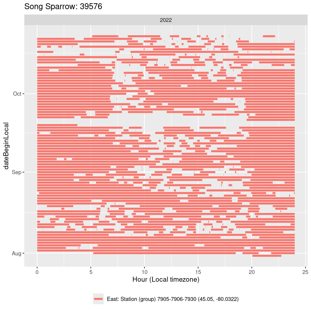
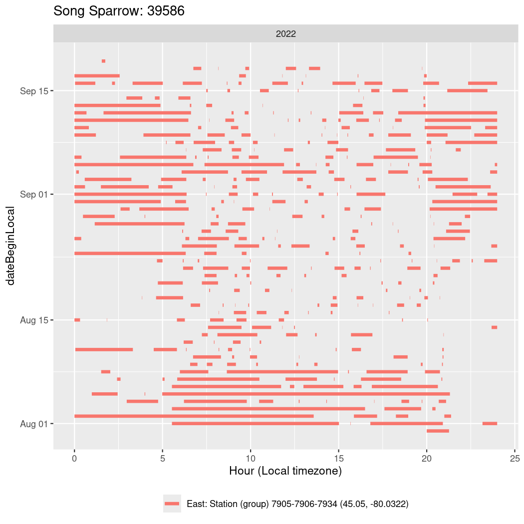
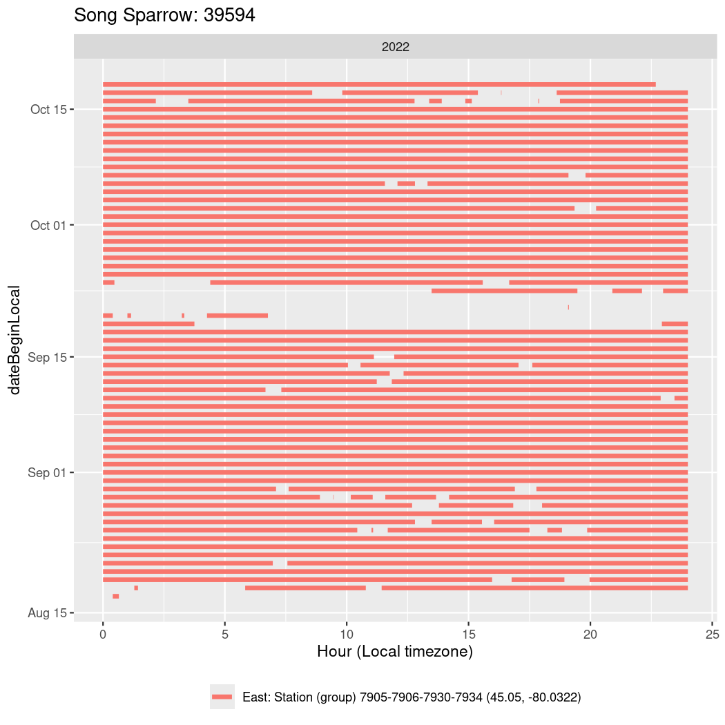
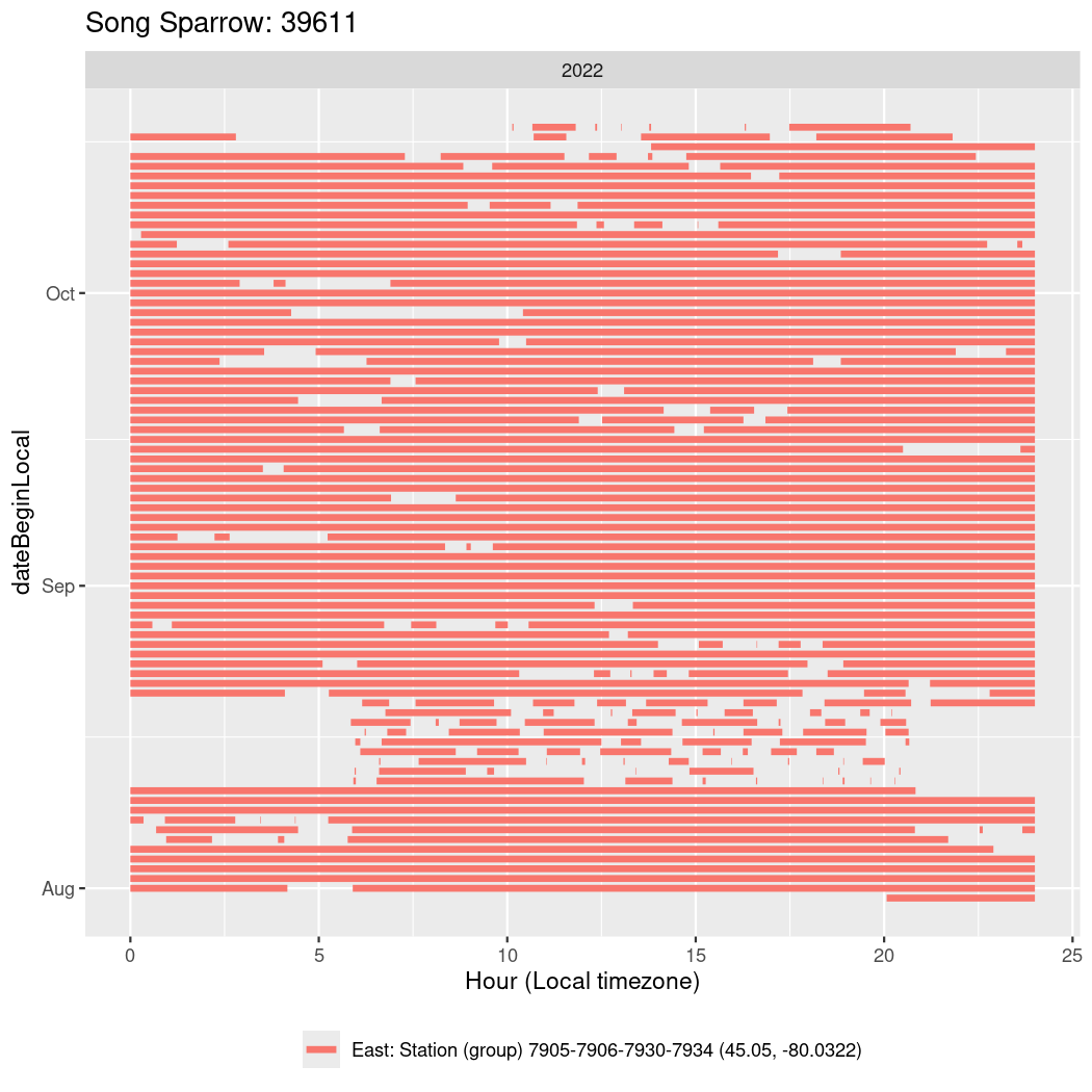
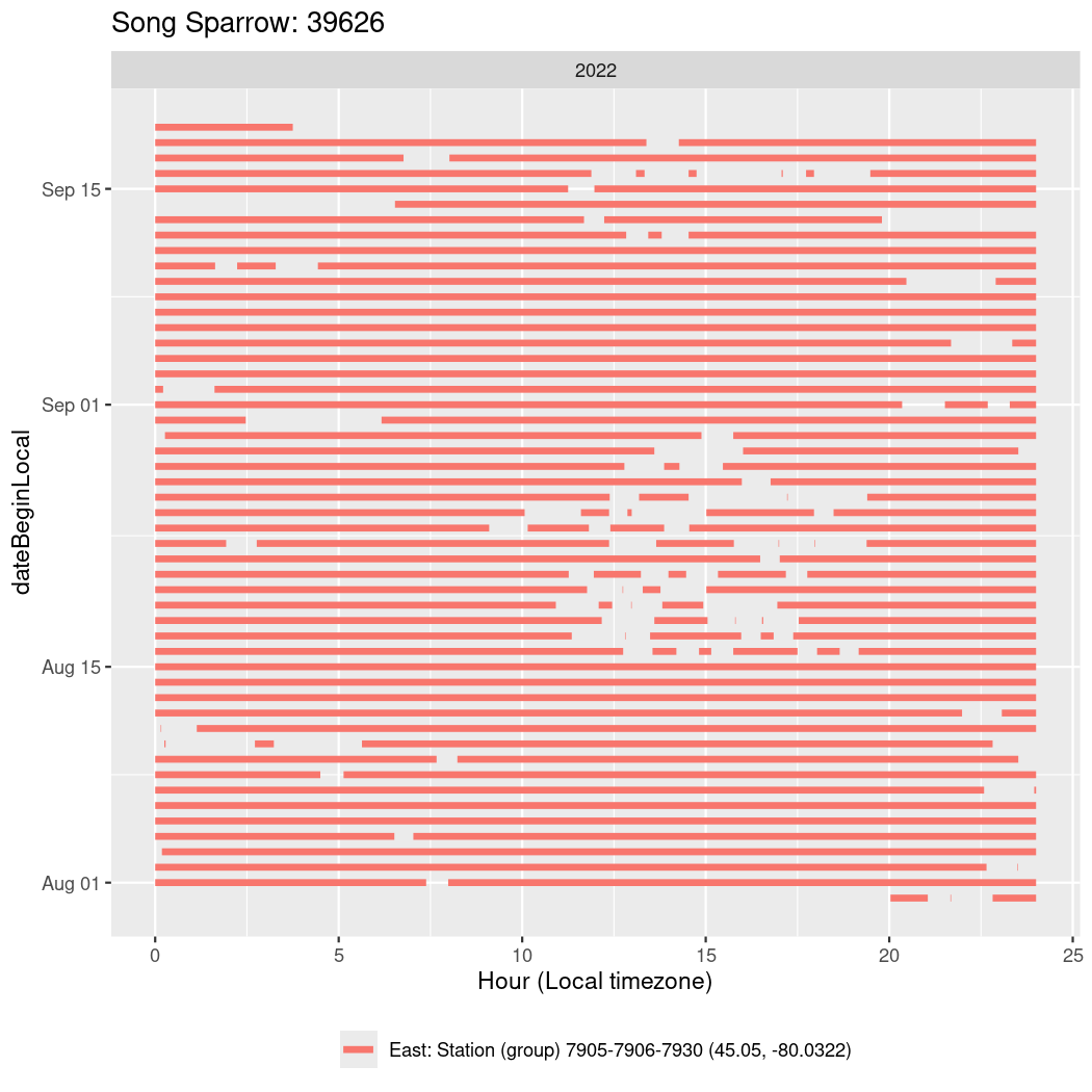
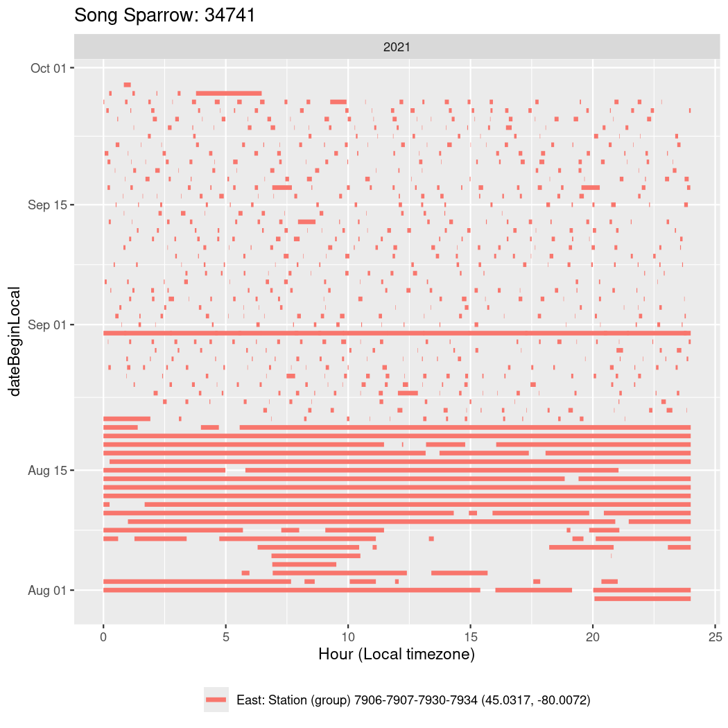
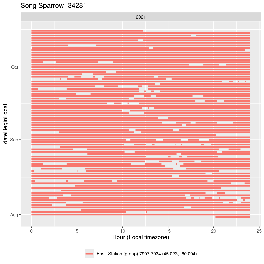
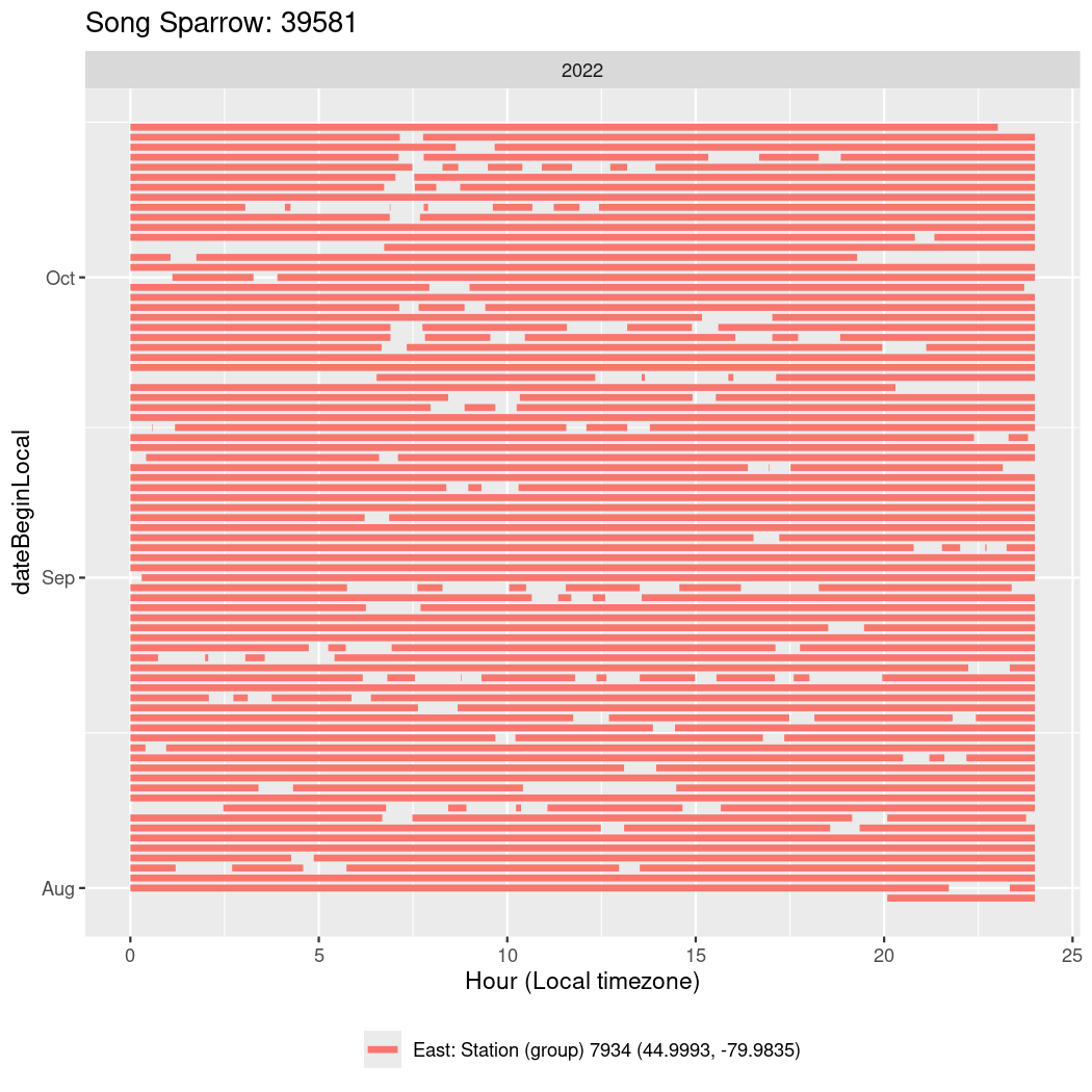
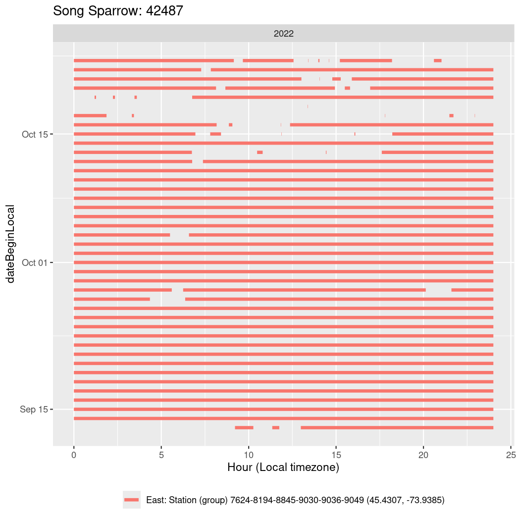
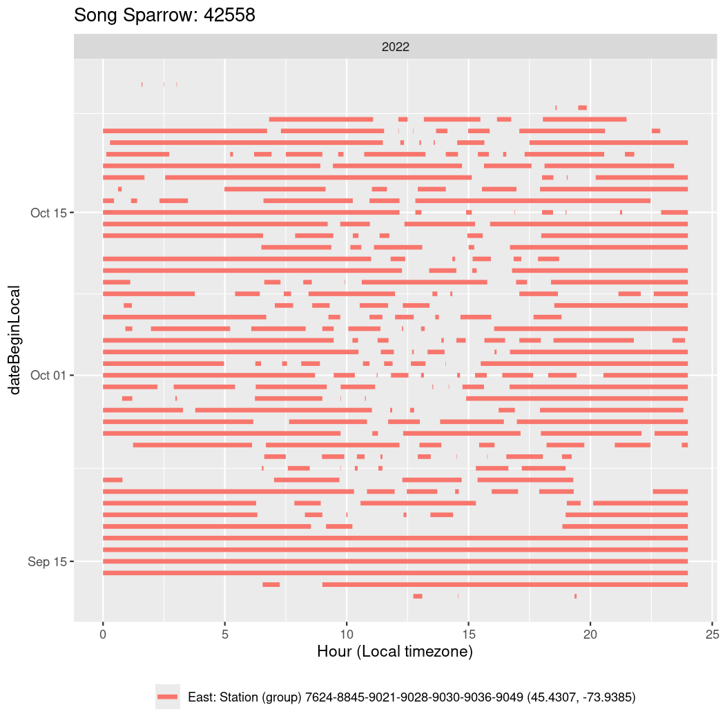
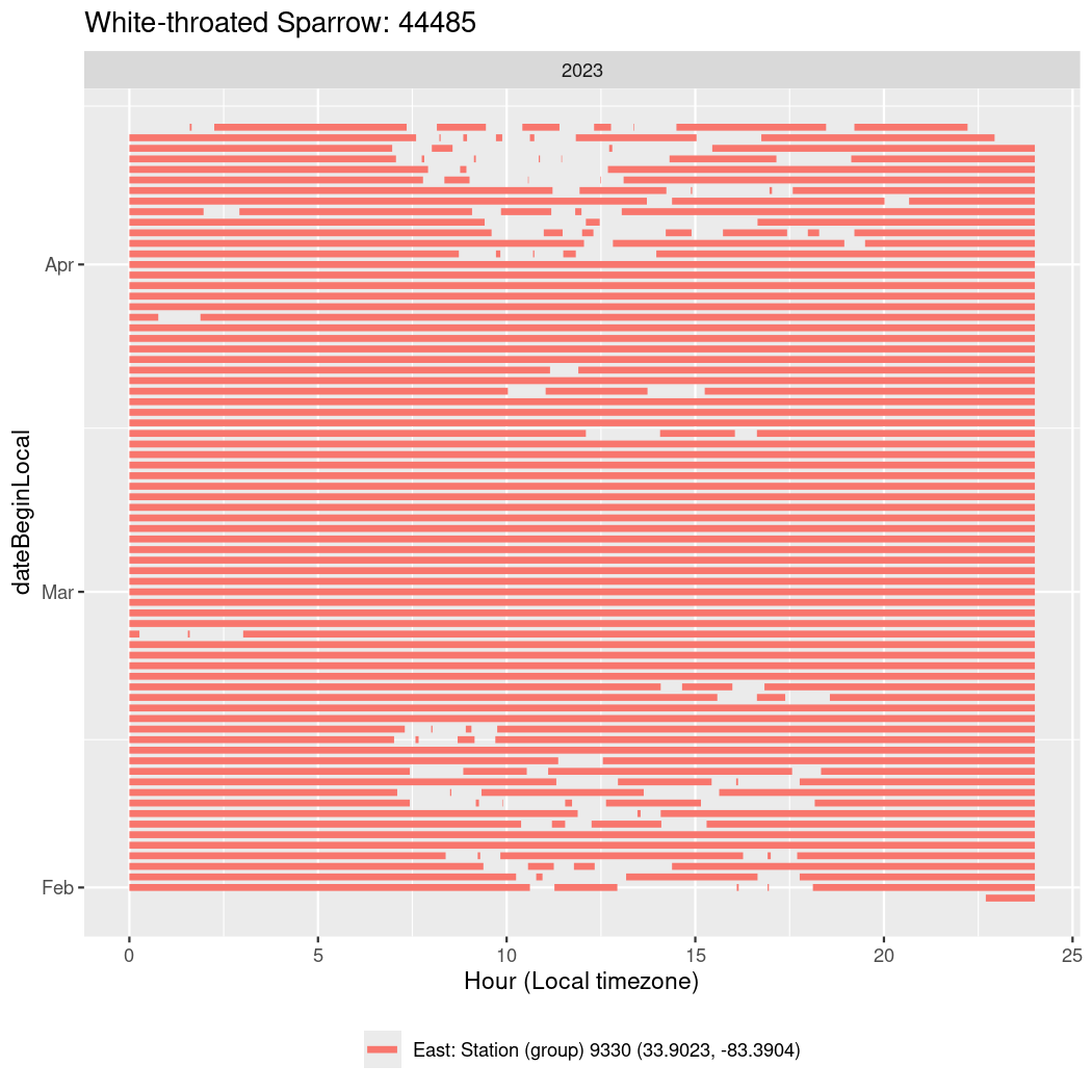
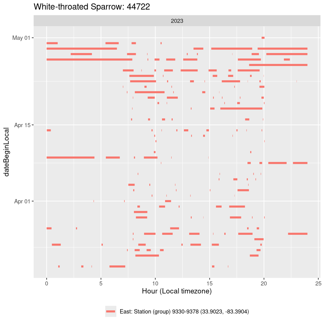
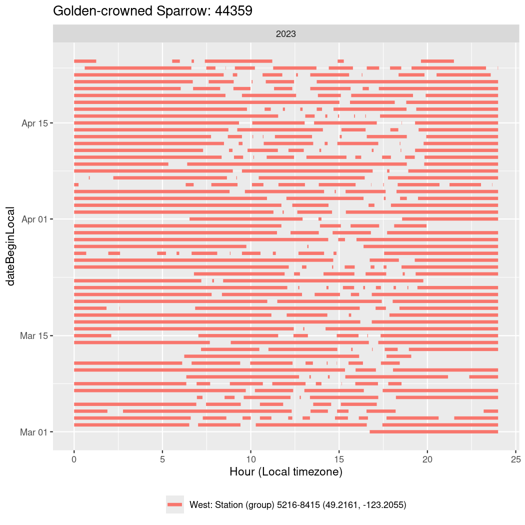
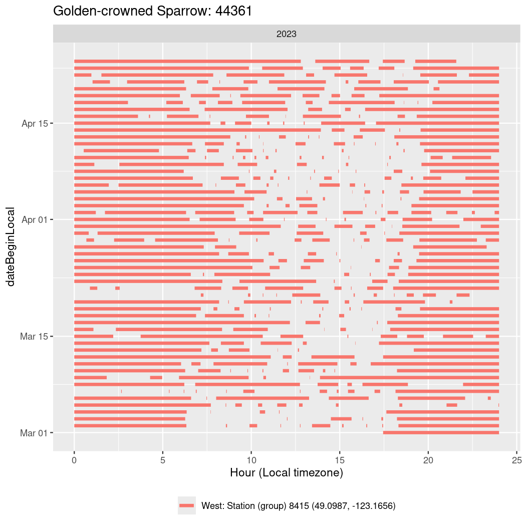
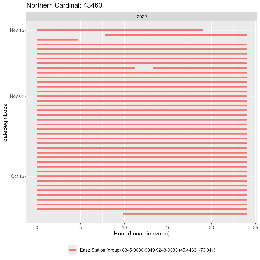
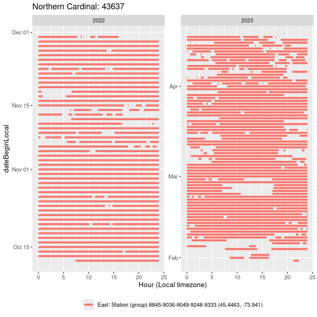
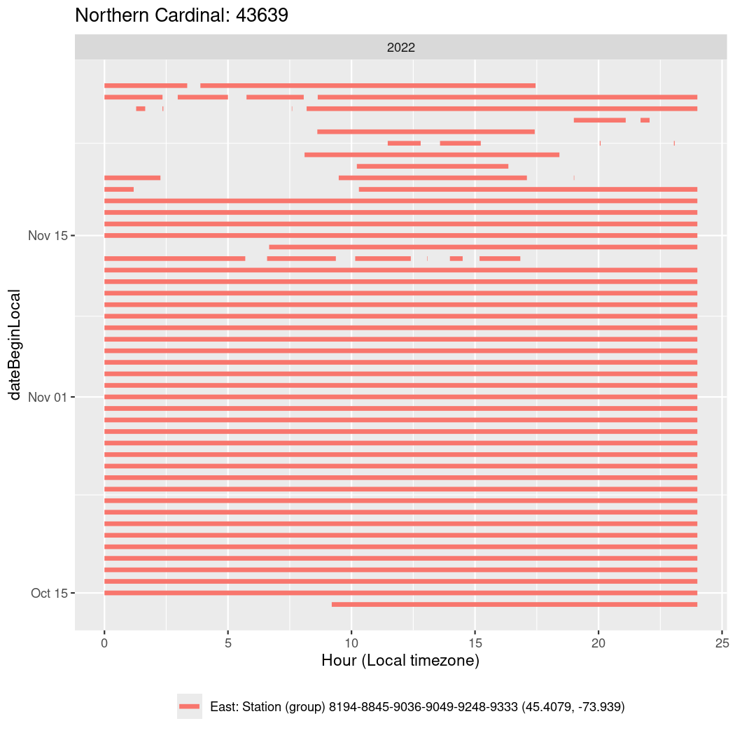
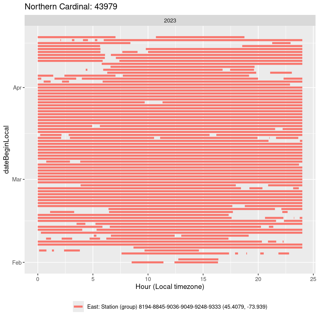
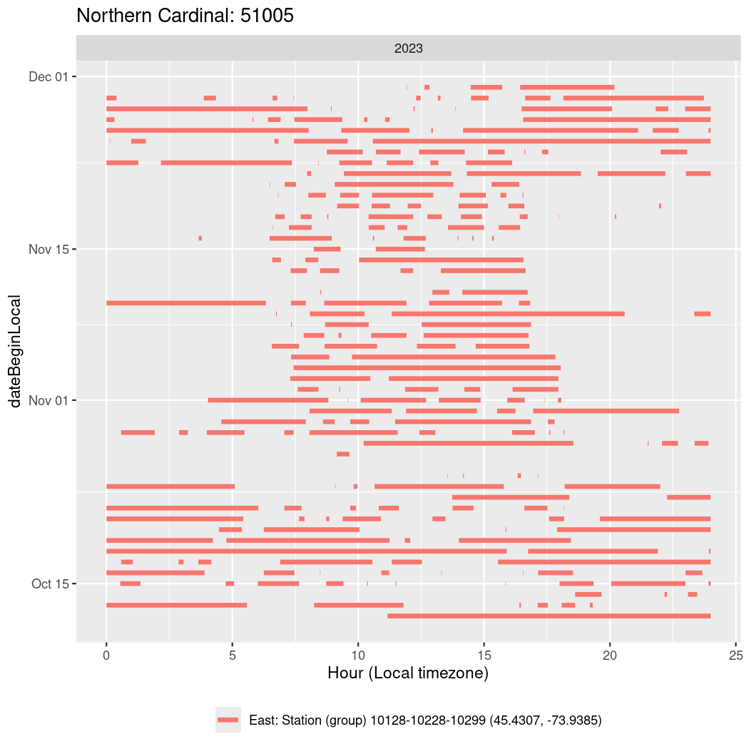
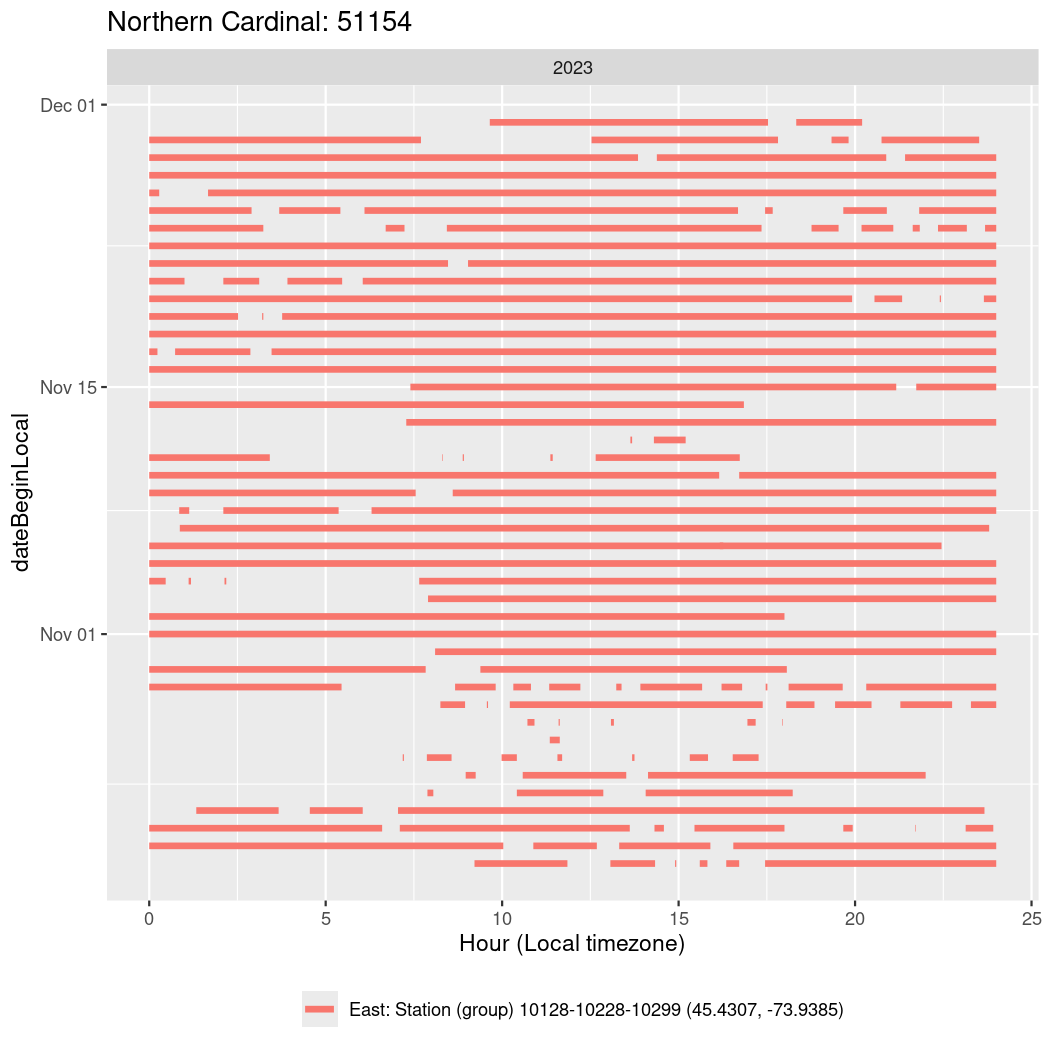
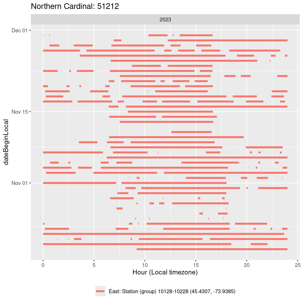
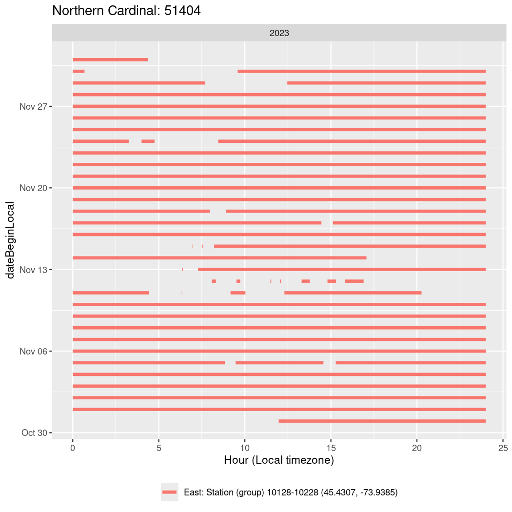
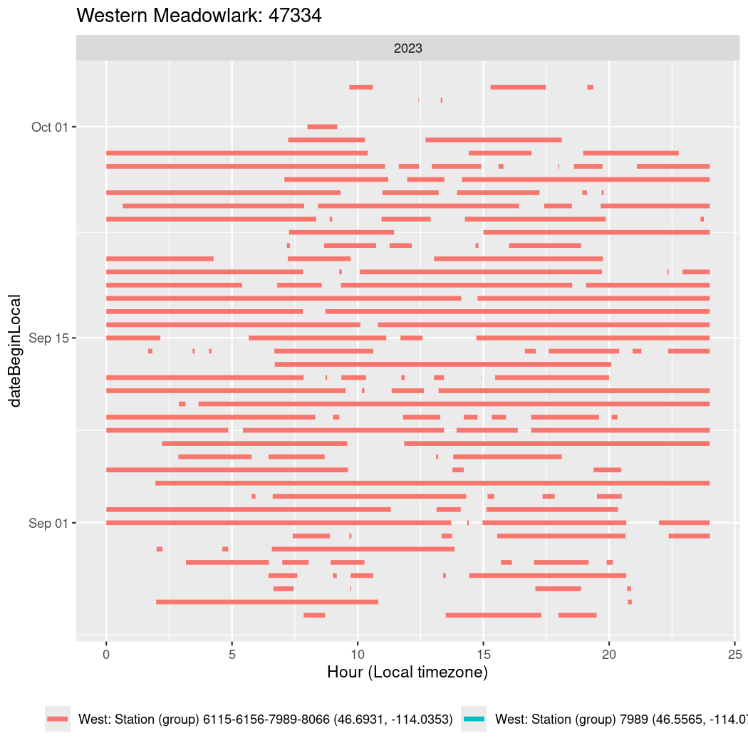
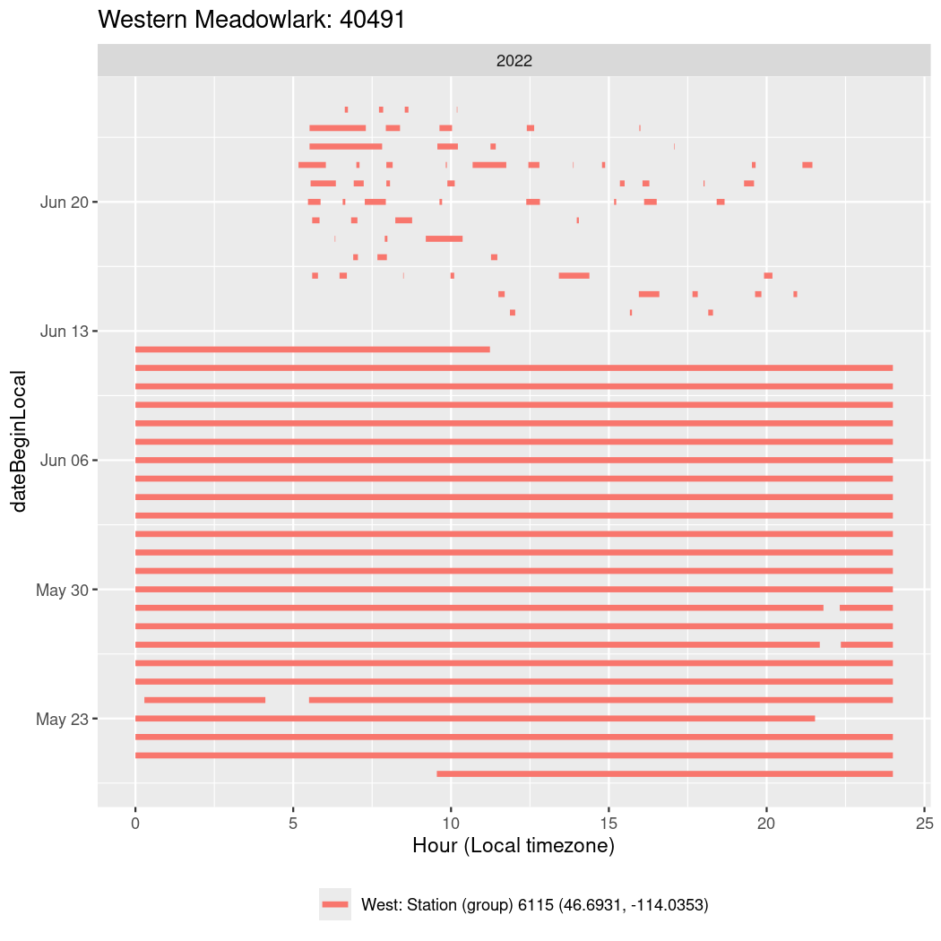
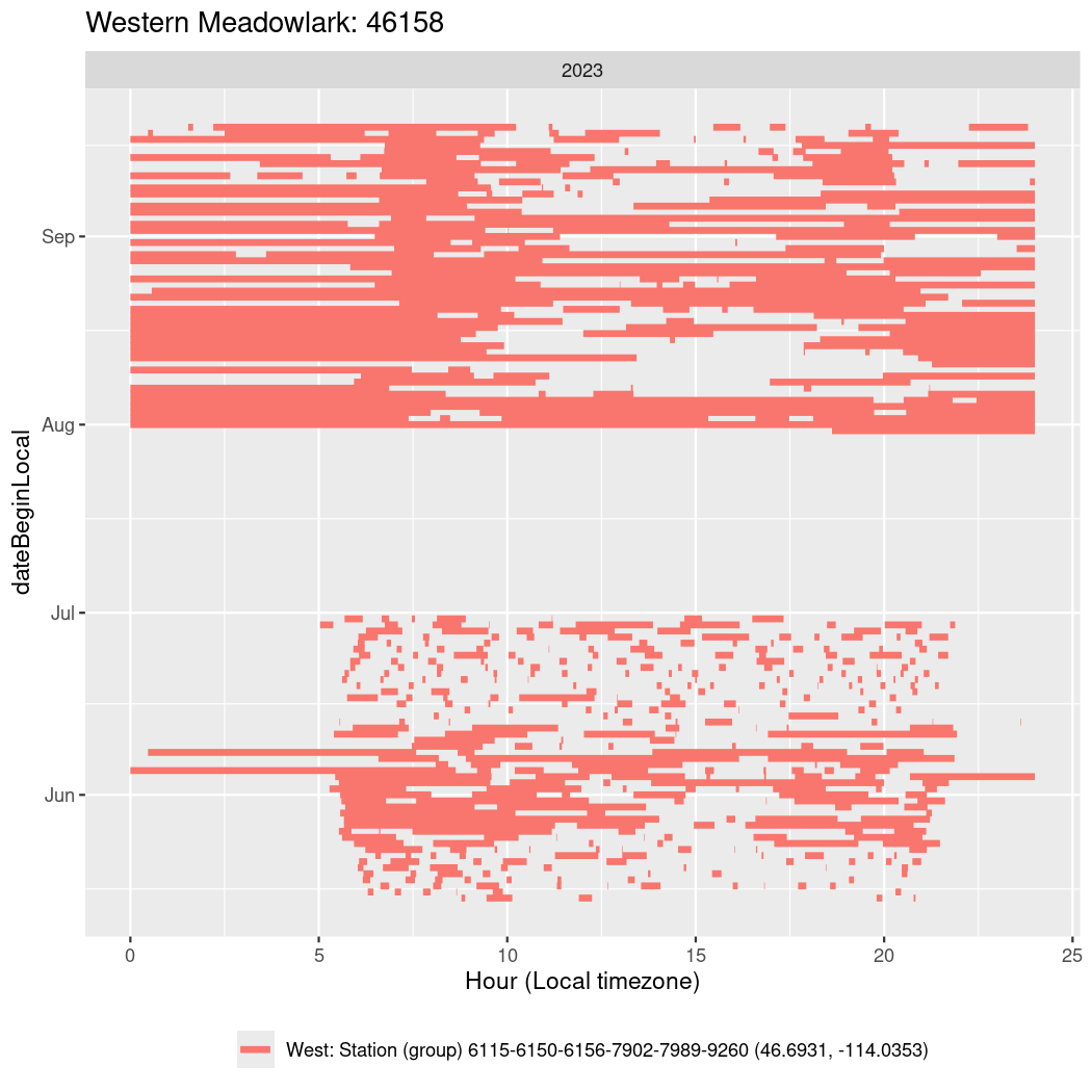
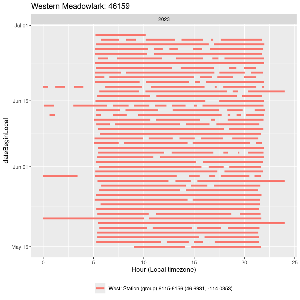
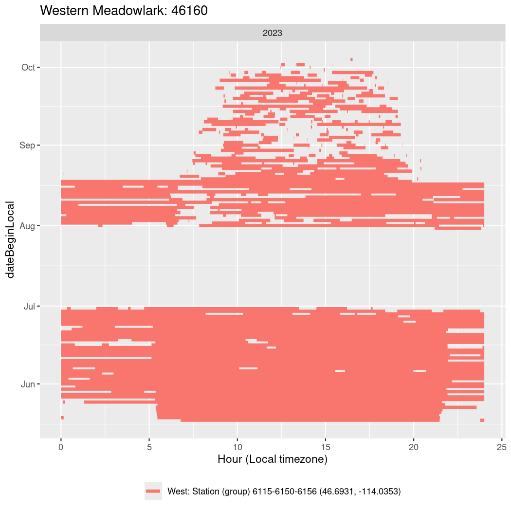
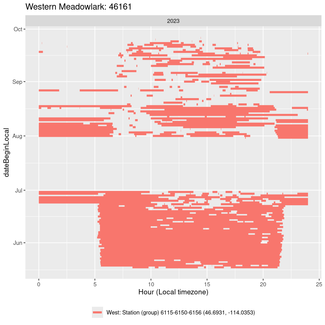
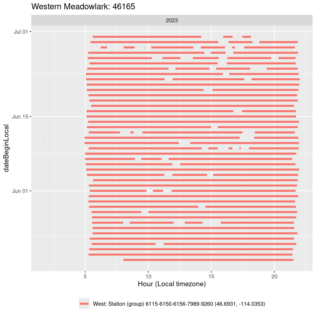
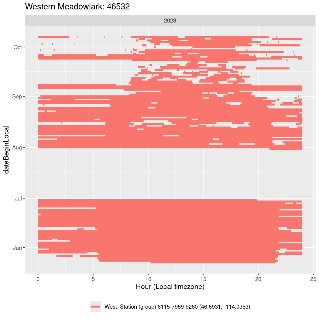
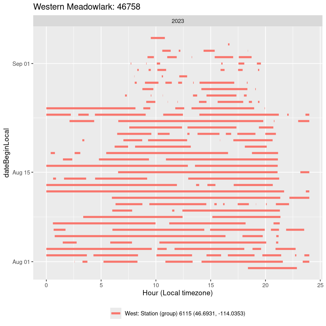
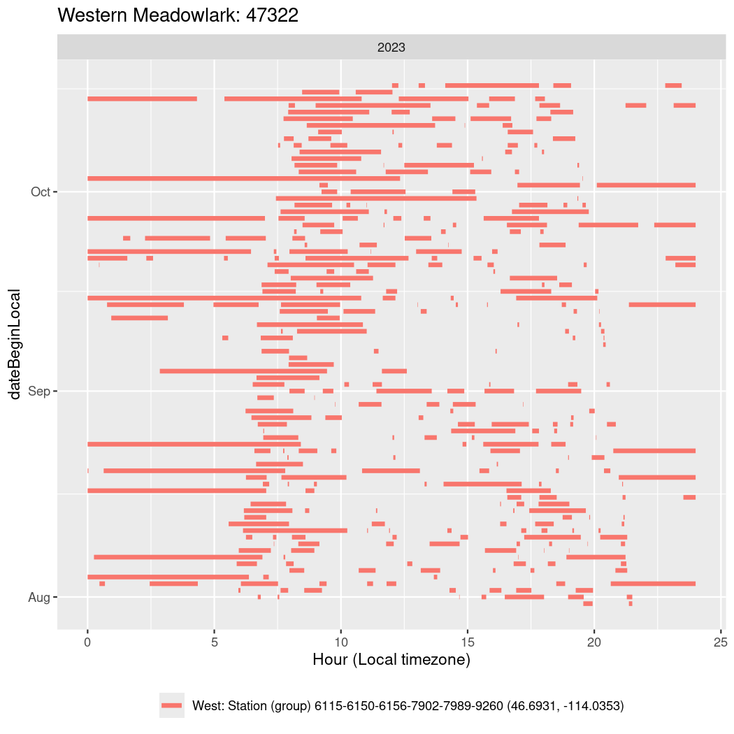
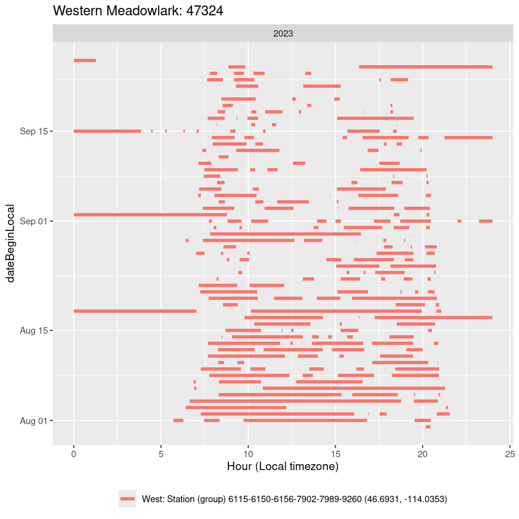
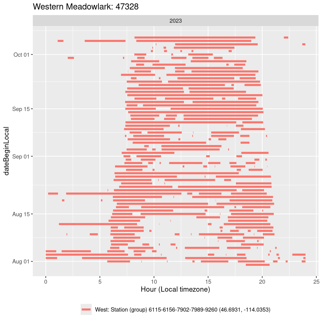
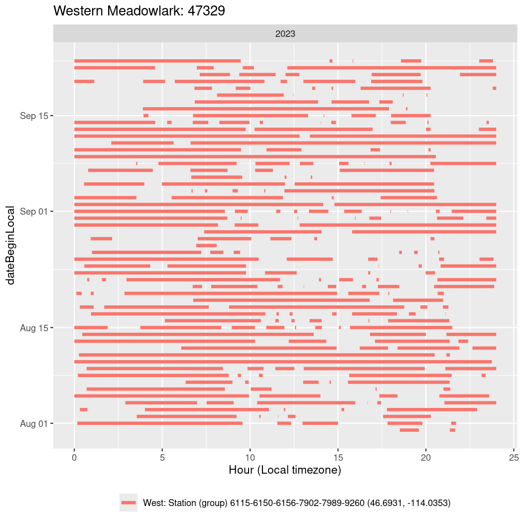
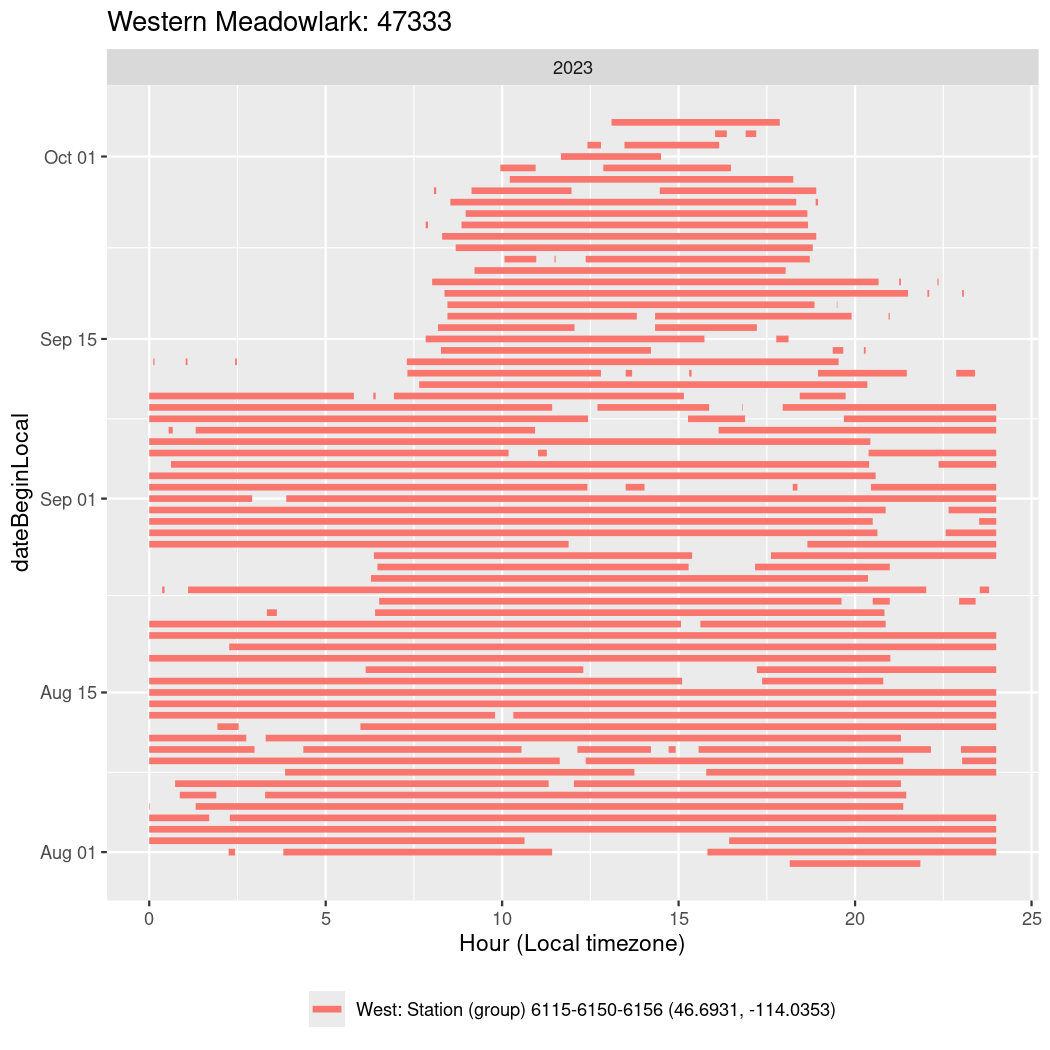
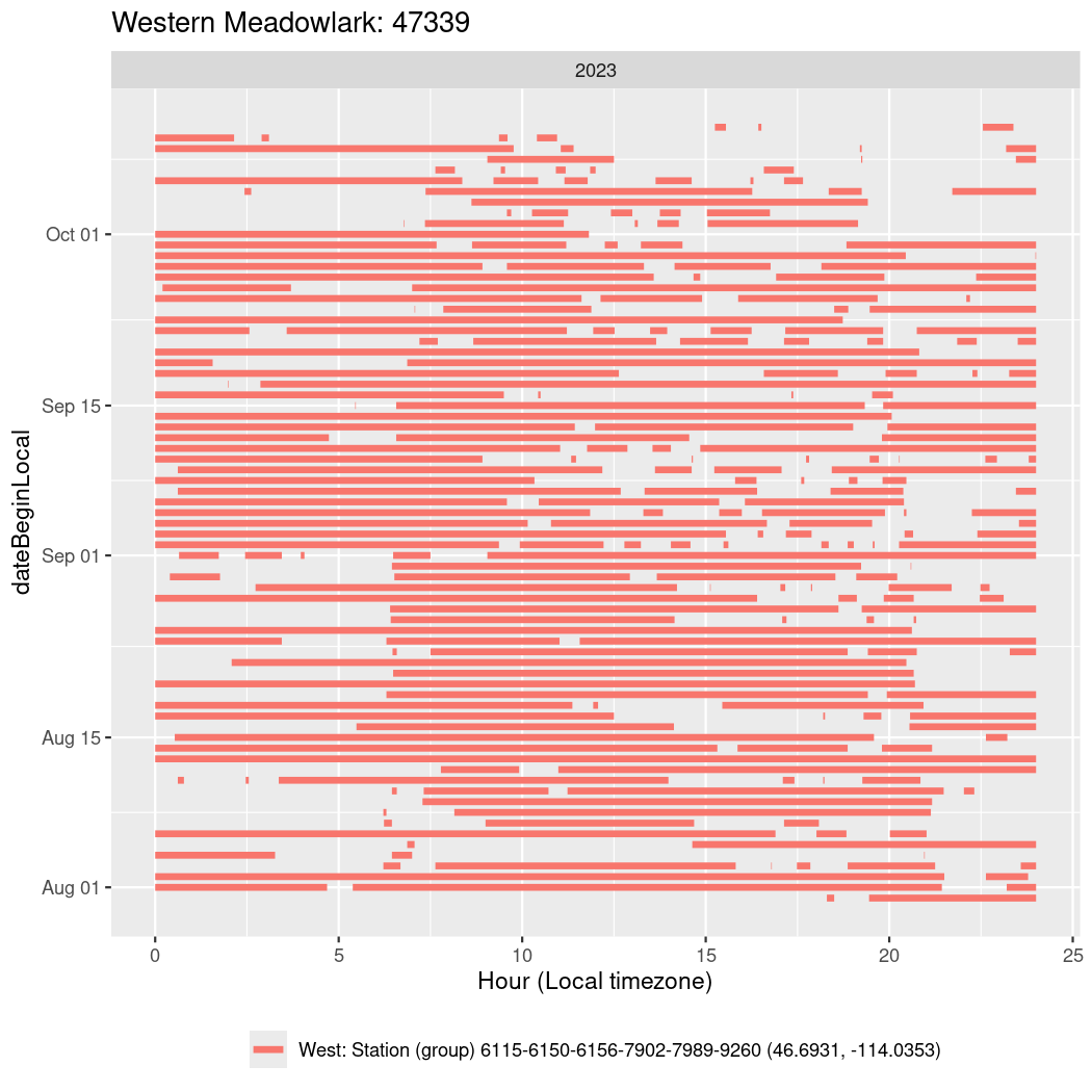
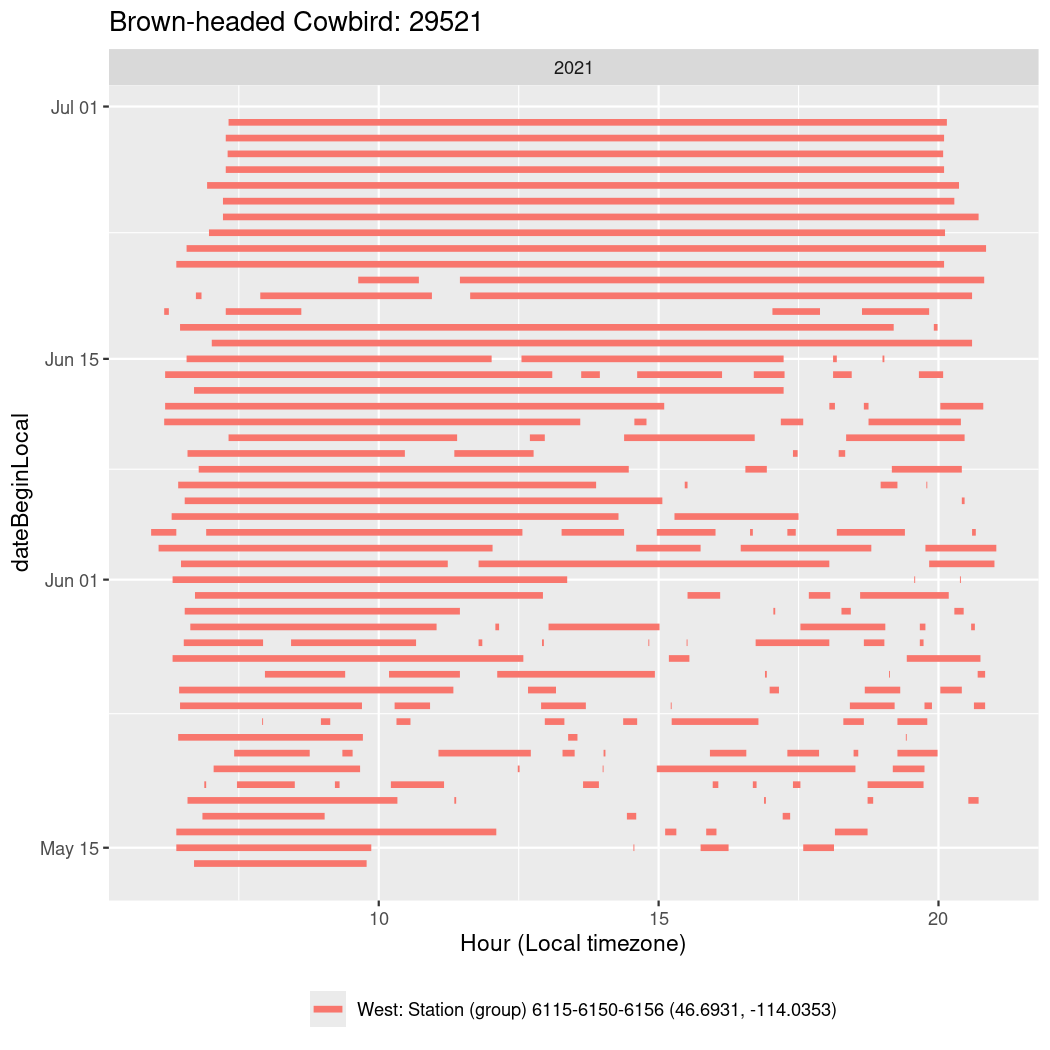
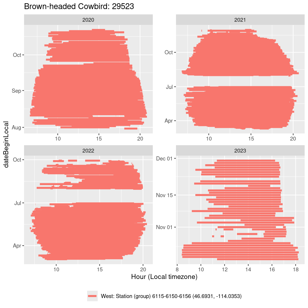
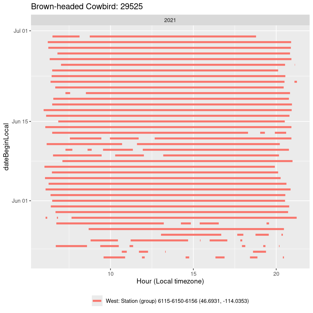
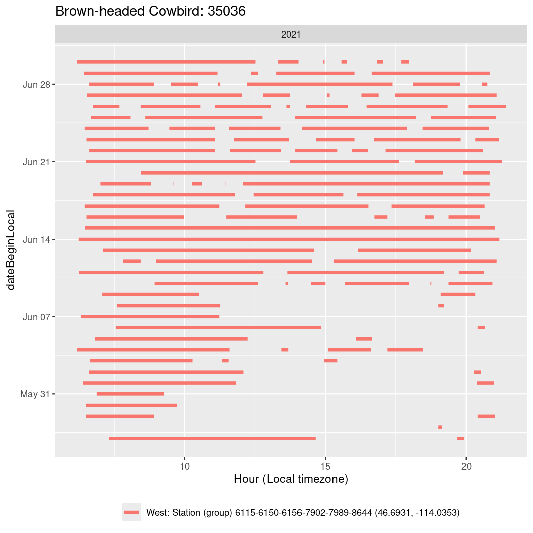
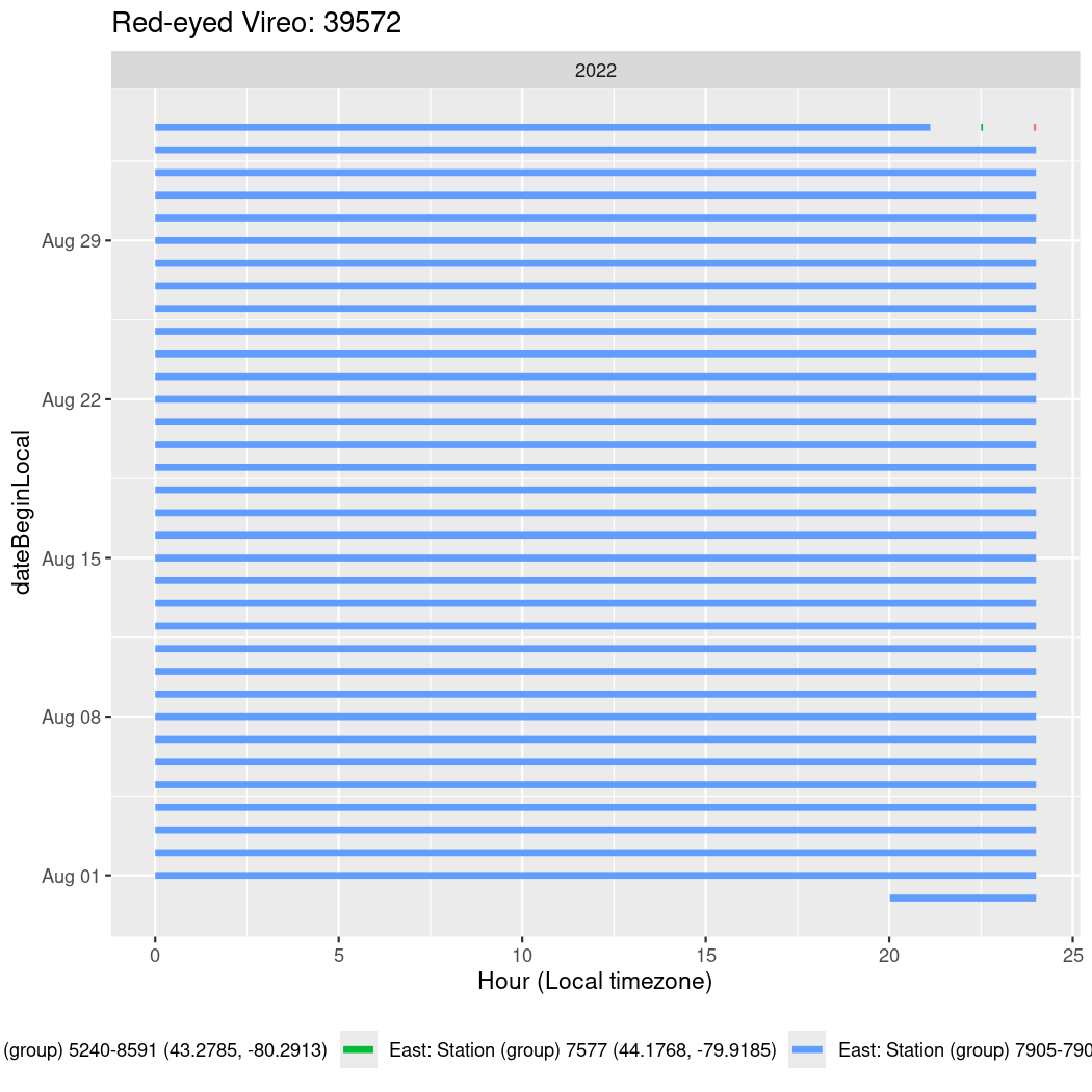
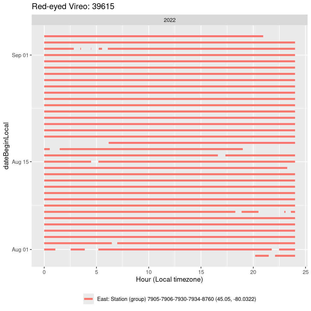
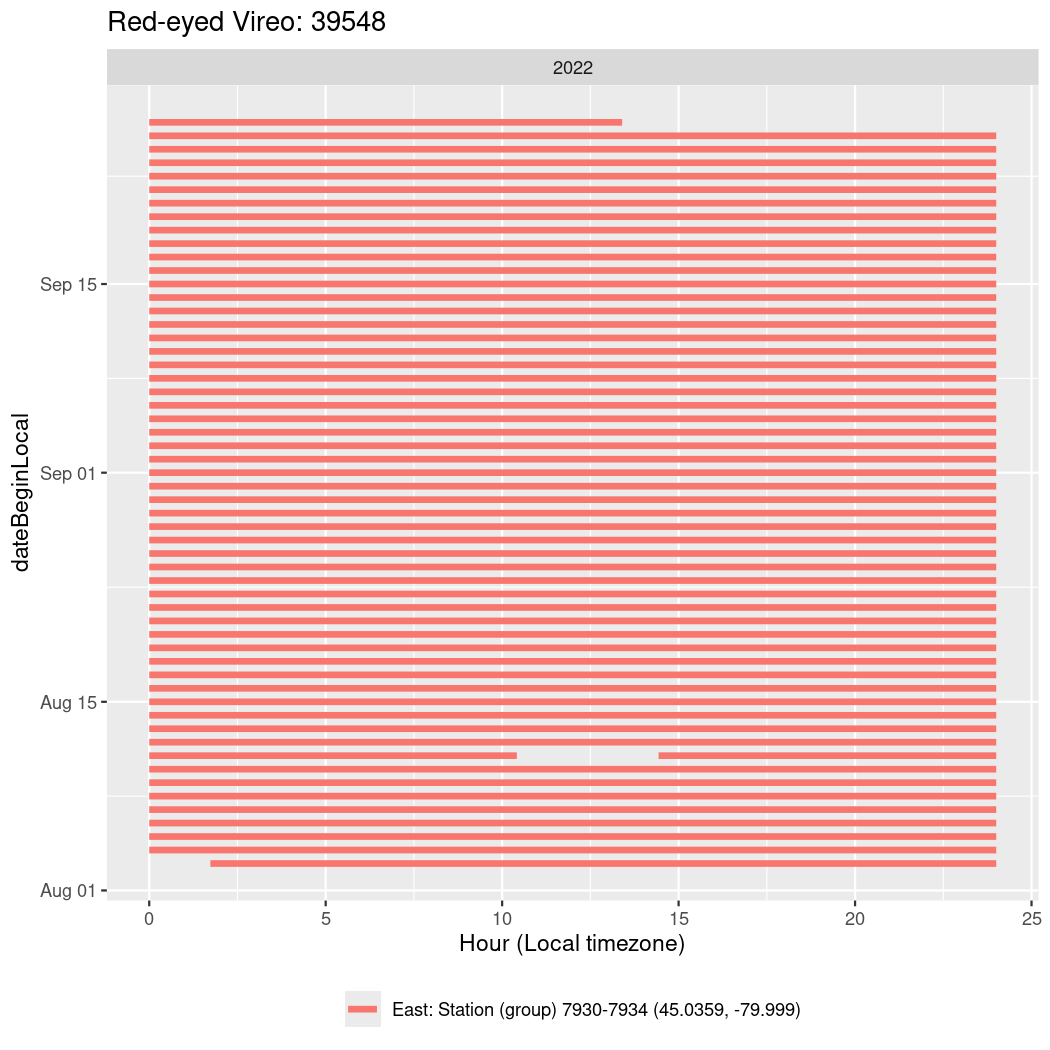
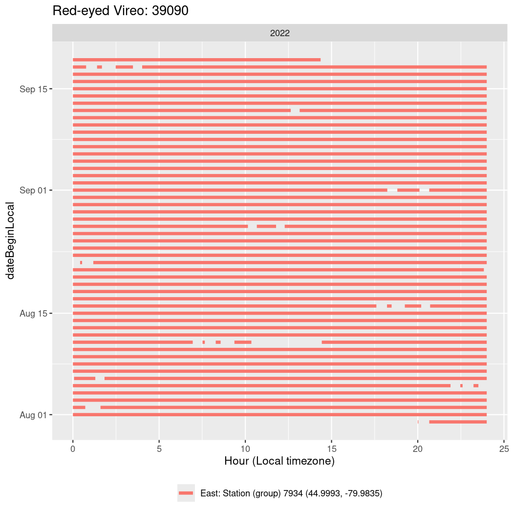
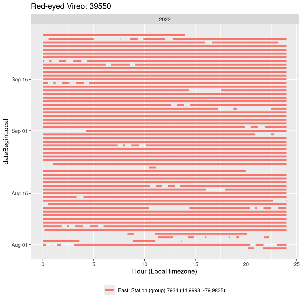
end = hour(timeEndLocal) + minute(timeEndLocal)/60)Next we’ll explore the activity (detections by a station over the course of the day).
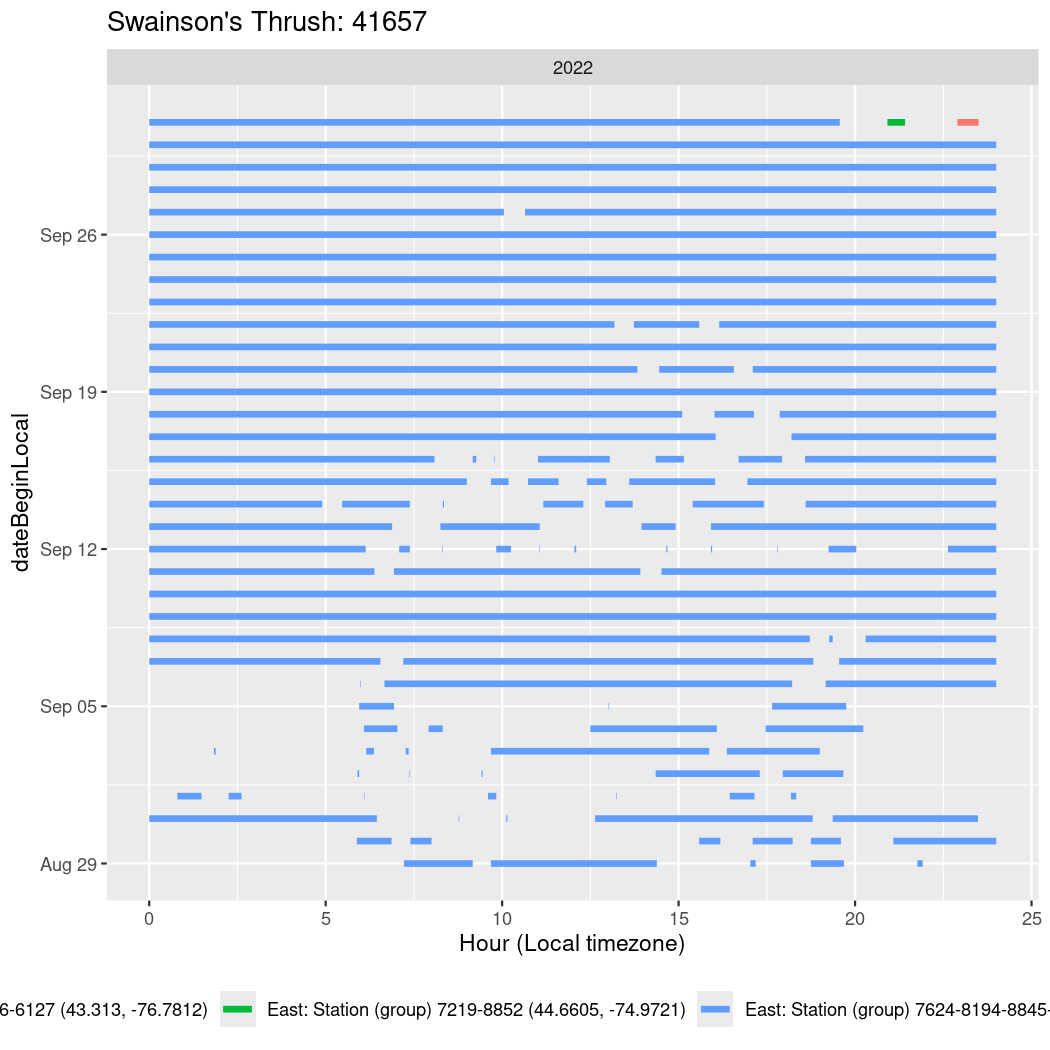
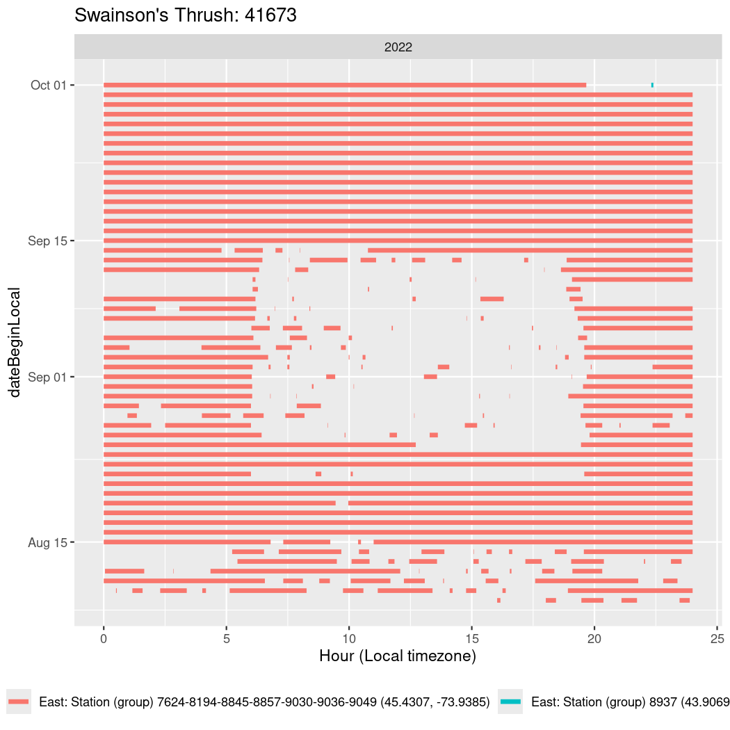
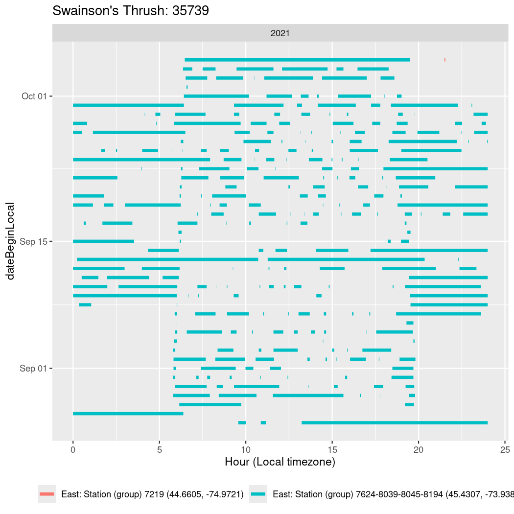
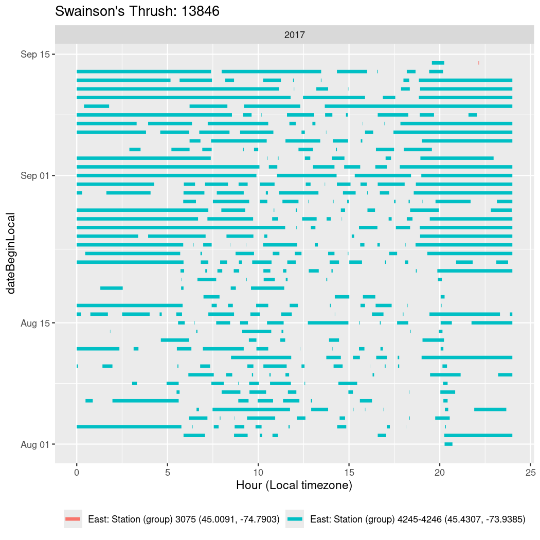
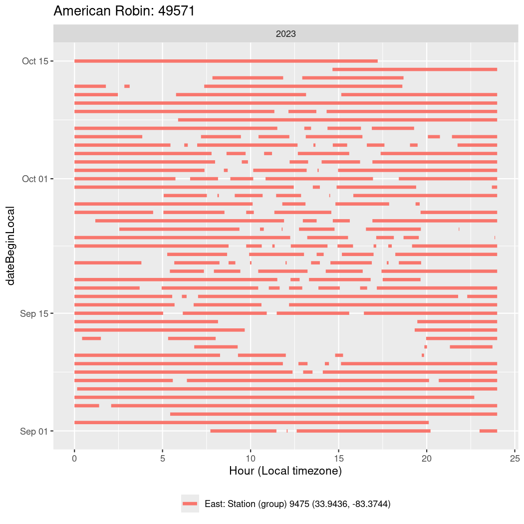
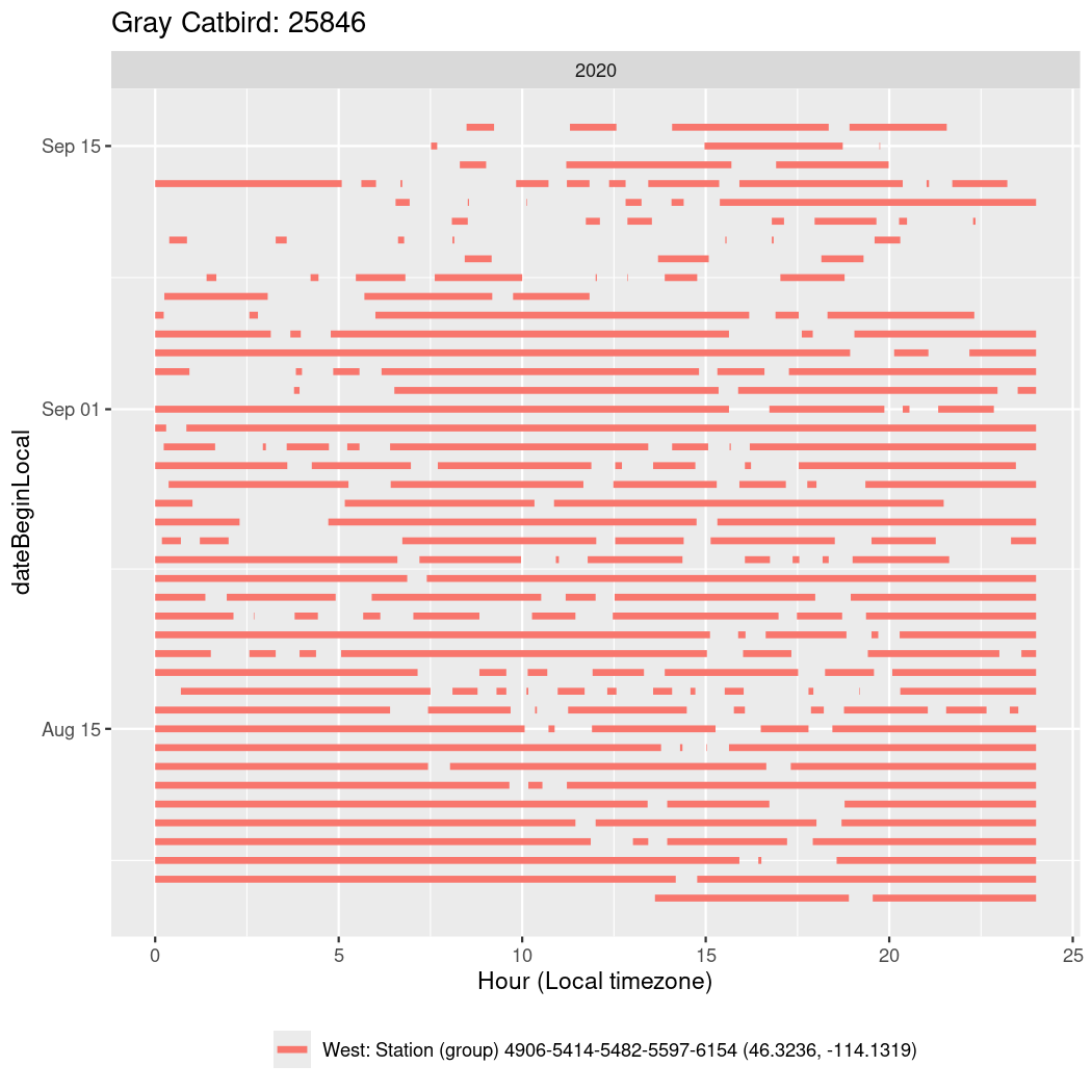
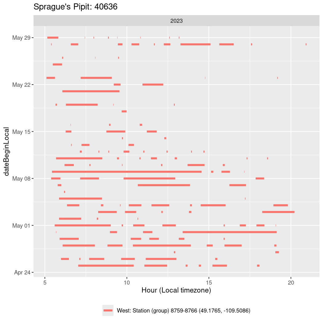
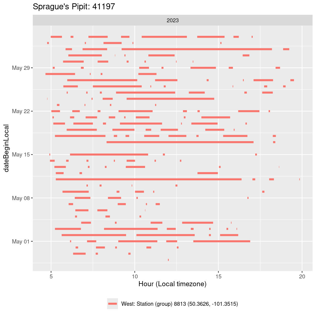
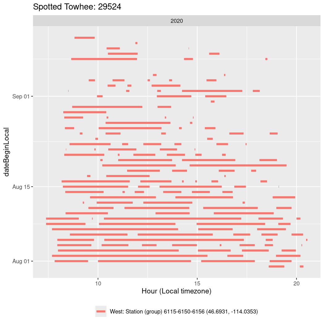
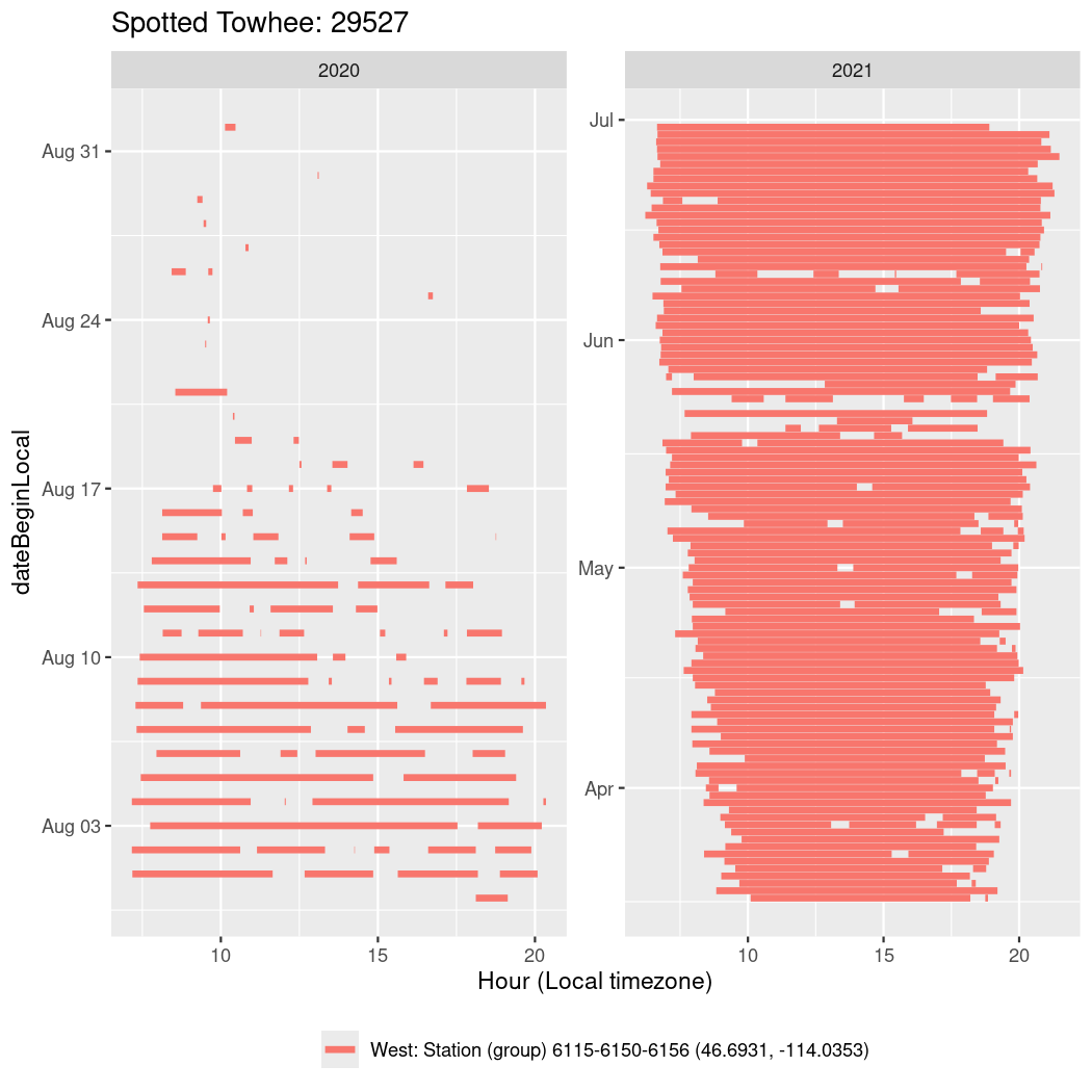
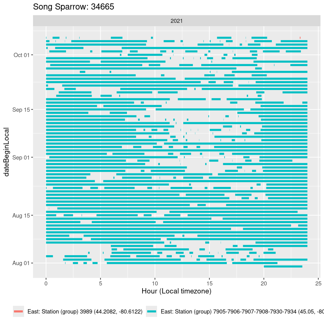
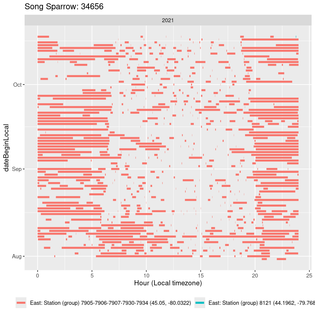
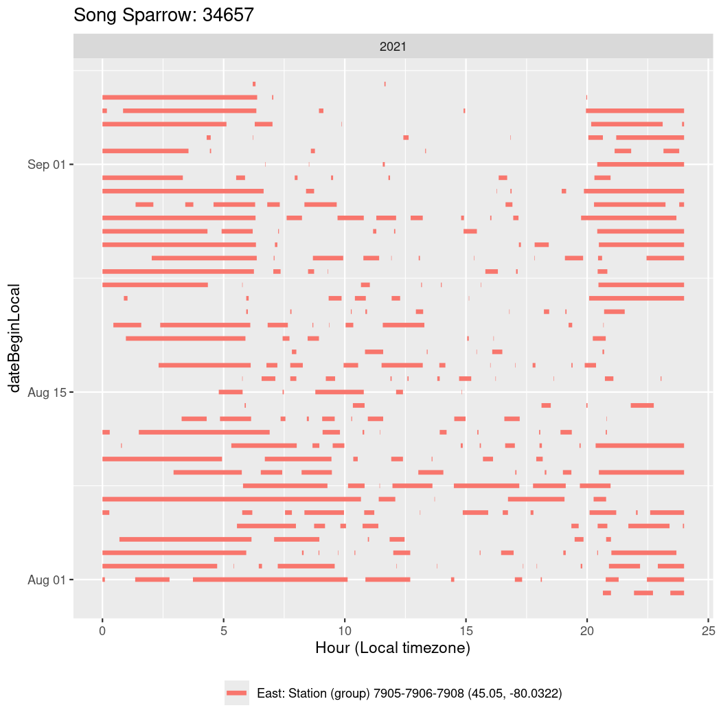
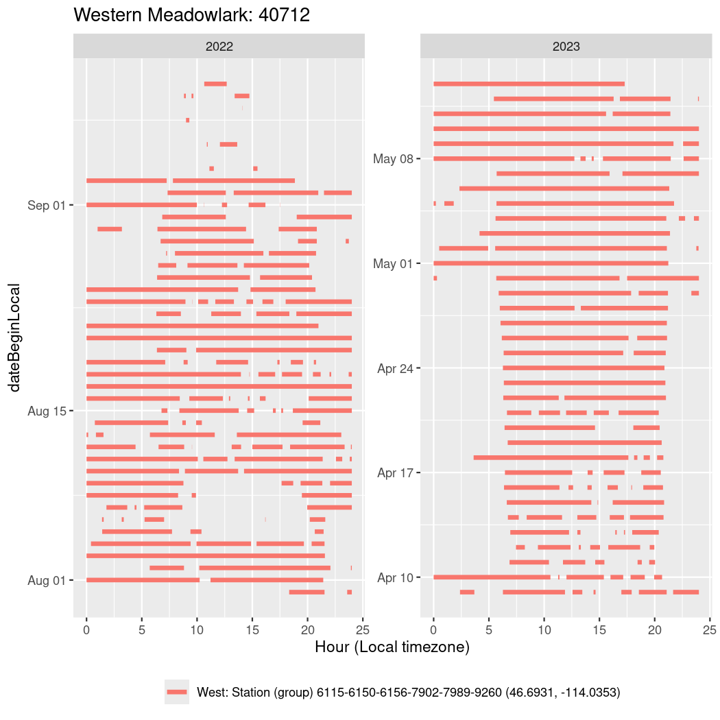
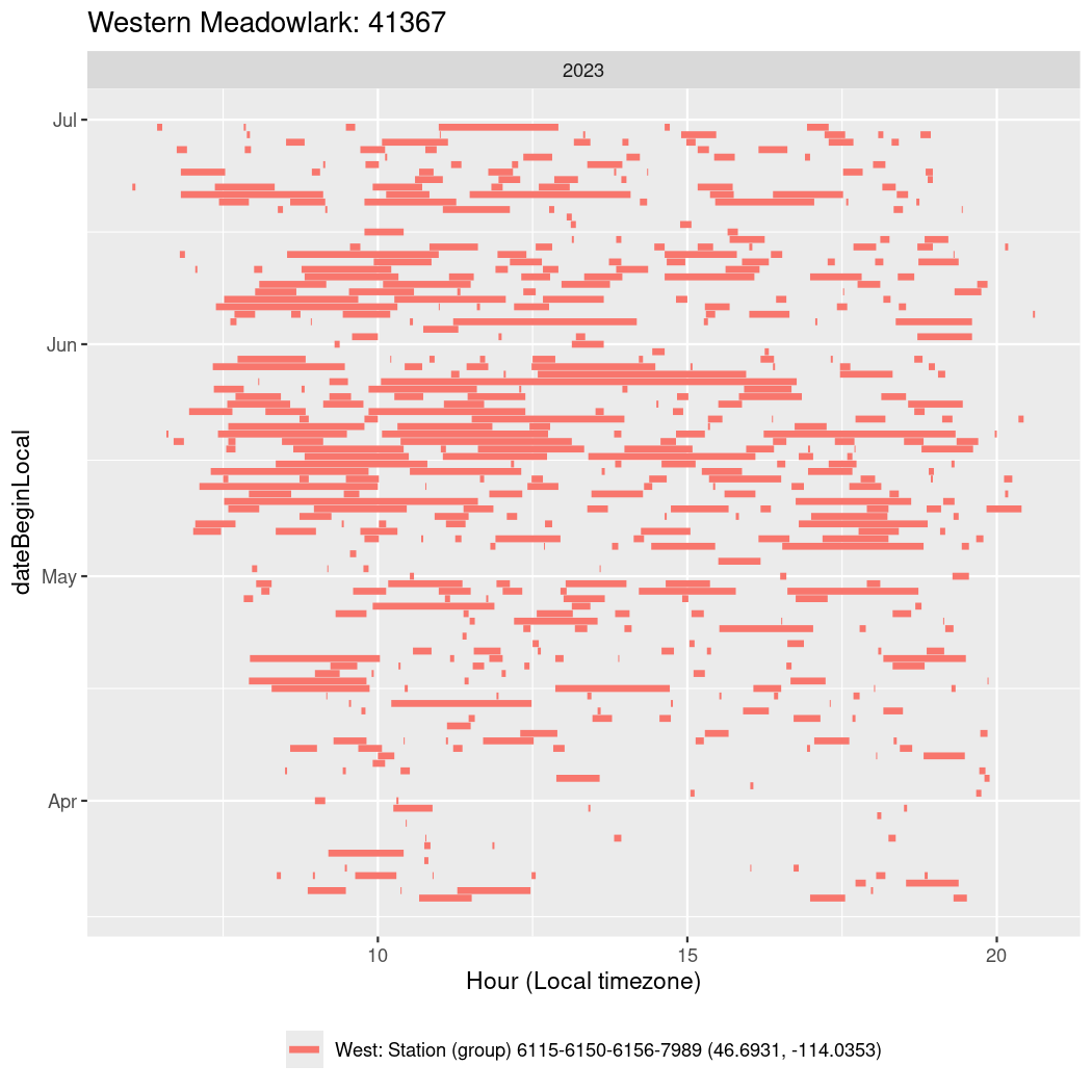
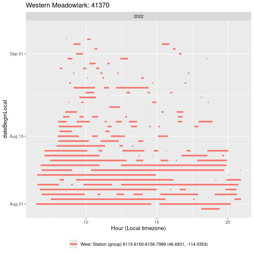
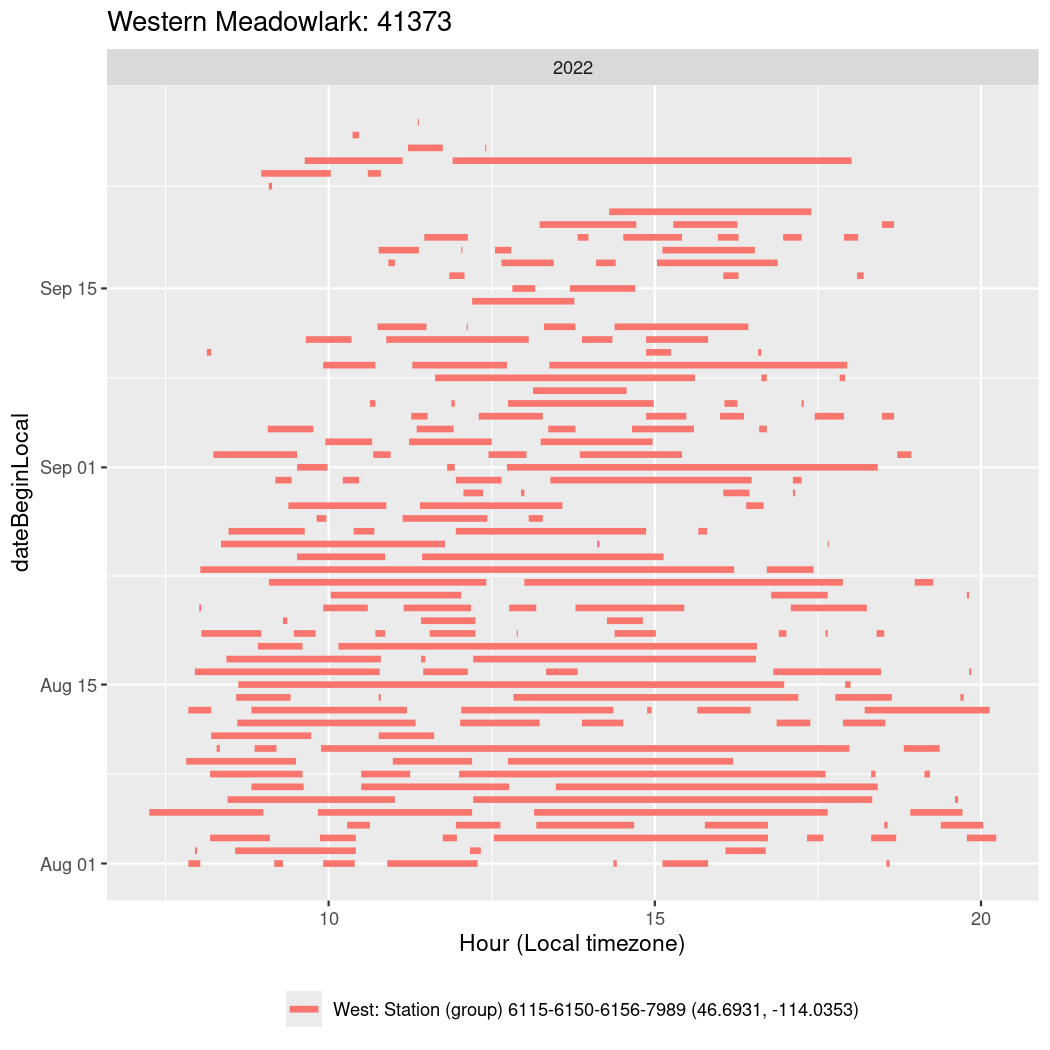
In these figures we’re looking at date along the Y axis and the time of day of bouts detected by a receiver on each day in local time along the X axis.
In both cases there is only one station that the birds are detected at (within the range of dates we’re exploring).
It suggests that there are times when these birds spend mornings near the receiver, but spend their nights or afternoons farther away before returning again for the evening (see the large patches of empty time between 10am and 8pm, especially in August and early September in the second figure. You can even see the funnel shape of the changing daylengths in the activity of these two birds.
Code
filter(b0, tagDeployID == 41224, dateBeginLocal > "2022-09-01", dateBeginLocal < "2023-01-01") |>
  ggplot(aes(x = start, xend = end, y = dateBeginLocal, colour = stn_group)) +
  geom_segment(linewidth = 1.5) +
  labs(x = "Hour (Local timezone)", title = "tagDeployID 41224 (Spotted Towhee)")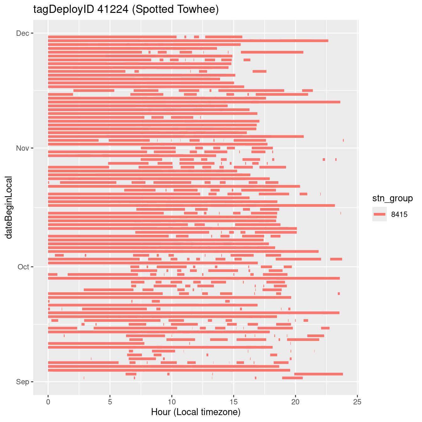
Code
filter(b0, tagDeployID == 41209, dateBeginLocal < "2022-12-01", dateBeginLocal > "2022-07-30") |>
  ggplot(aes(x = start, xend = end, y = dateBeginLocal, colour = stn_group)) +
  geom_segment(linewidth = 1.5) +
  labs(x = "Hour (Local timezone)", title = "tagDeployID 41224 (Spotted Towhee)")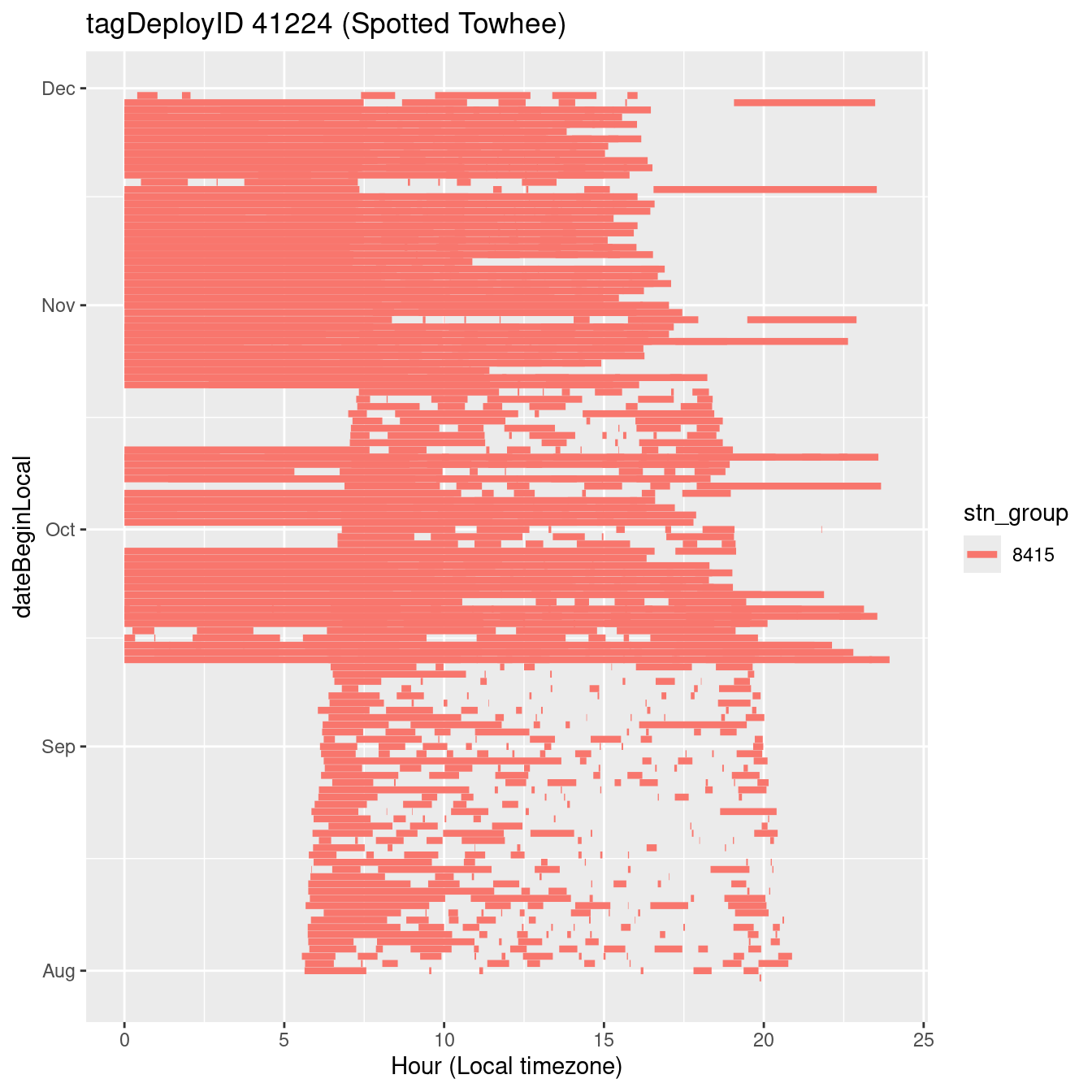
Create data set for exploration
Datasets created:
The above exploration revealed some interesting patterns. While we don’t have time in this round of the project to get into them in detail, we can create a data set for exploration.
We’ll filter the bout-level data to include only periods of time for individuals when they spent more than 30 days at a specific station (without being detected at other stations in between). This may omit some which are hanging out in a local area and are being recorded by multiple stations, but at least gives us a starting point.
:::{.callout-tip} #### Note We filter by ID and date, not by station, so figures will show birds at multiple stations if they
include <- daily_bouts |>
  arrange(tagDeployID, dateBeginLocal) |>
  mutate(same_stn1 = lead(stn_group, default = "X") == stn_group &
           difftime(lead(dateBeginLocal, default = ymd("2099-01-01")), dateBeginLocal, units = "days") < 3,
         same_stn2 = lag(stn_group, default = "X") == stn_group &
           difftime(dateBeginLocal, lag(dateBeginLocal, default = ymd("1900-01-01")), units = "days") < 3,
         .by = "tagDeployID") |>
  filter(!(!same_stn1 & !same_stn2)) |>
  mutate(start = same_stn1 & !same_stn2,
         end = !same_stn1 & same_stn2) |>
  mutate(group = cumsum(start), .by = "tagDeployID") |>
  mutate(n = n(),  min = min(dateBeginLocal), max = max(dateBeginLocal),
         .by = c("tagDeployID", "group")) |>
  filter(n > 20, difftime(max, min, units = "days") > 30) |>
  select(tagDeployID, stn_group, group, n, min, max) |>
  distinct()

circadian <- bouts_split |>
  mutate(year = year(dateBeginLocal)) |>
  semi_join(include, by = join_by("tagDeployID", between(dateBeginLocal, min, max))) |>
  mutate(start = hour(timeBeginLocal) + minute(timeBeginLocal)/60,
         end = hour(timeEndLocal) + minute(timeEndLocal)/60,
         end = if_else(end == 0, 24, end), # Account for days where the bird was detected over midnight
         stn_nice = paste0(
           if_else(recvDeployLon < -94.96, "West", "East"),
           ": Station (group) ", stn_group,
           " (", round(recvDeployLat, 4), ", ", round(recvDeployLon, 4), ")")) |>
  arrange(speciesID, recvDeployLon)

write_csv(select(circadian, -"stn_nice"), "Data/03_Final/summary_circadian_bouts.csv")
Broad exploration
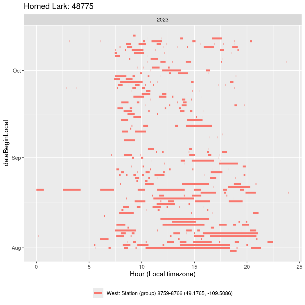
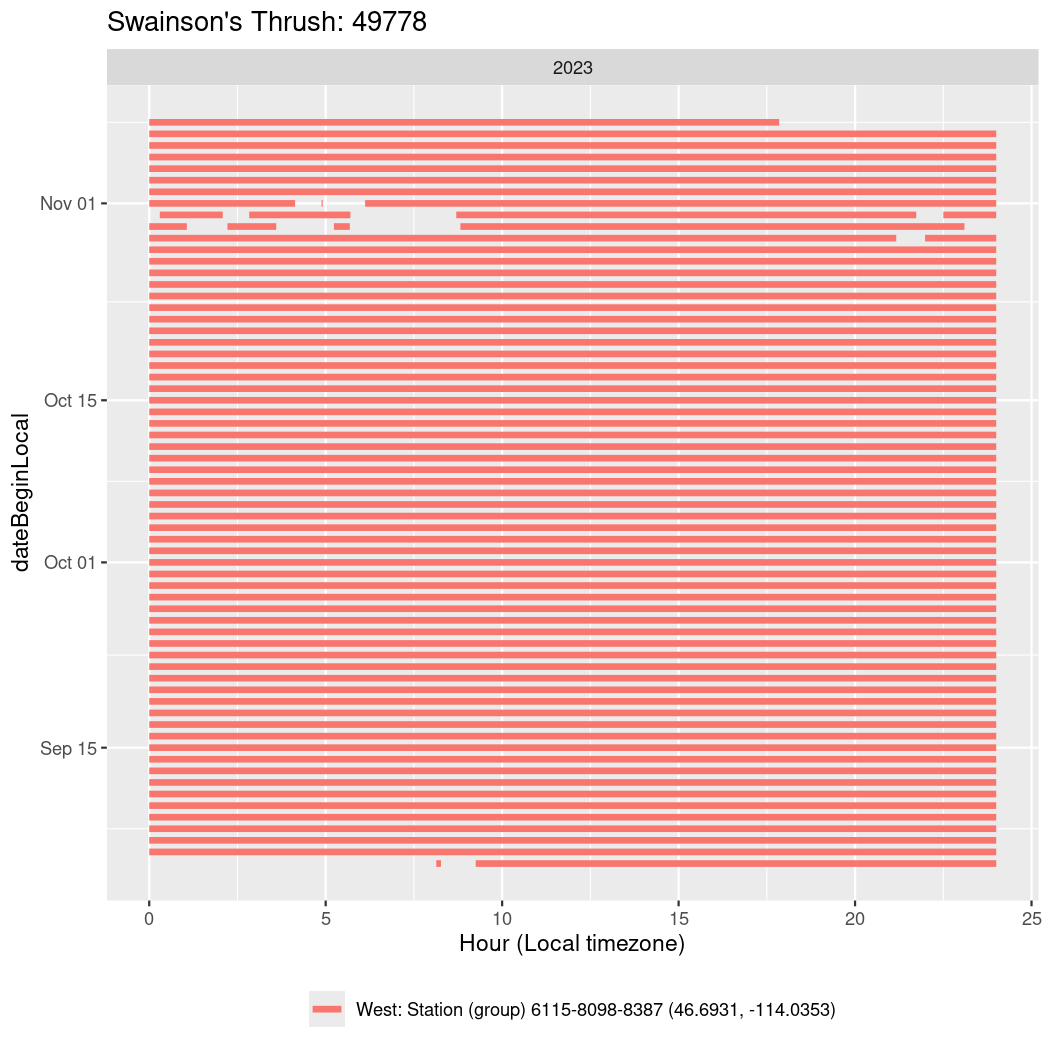
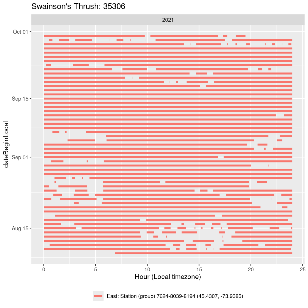
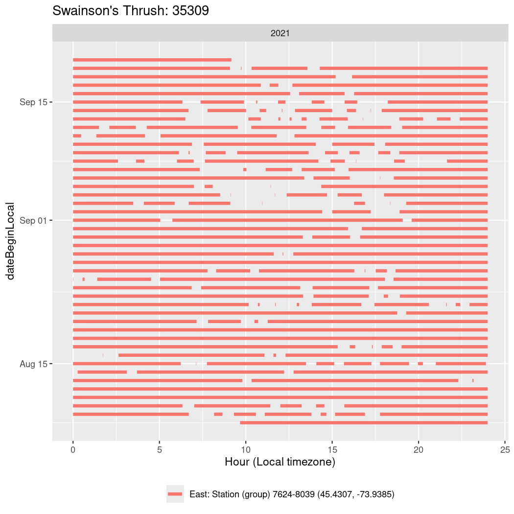
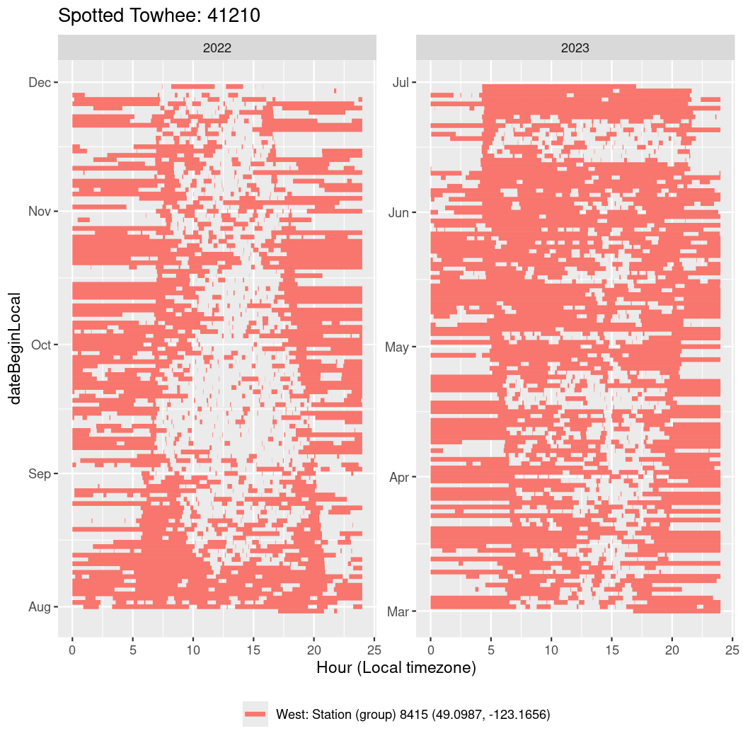
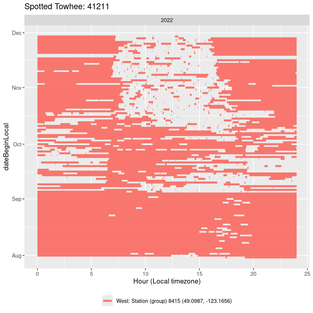
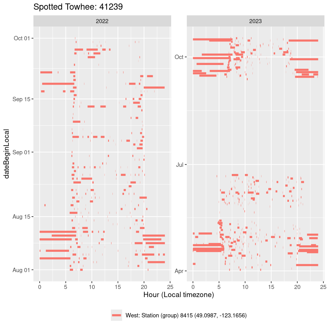
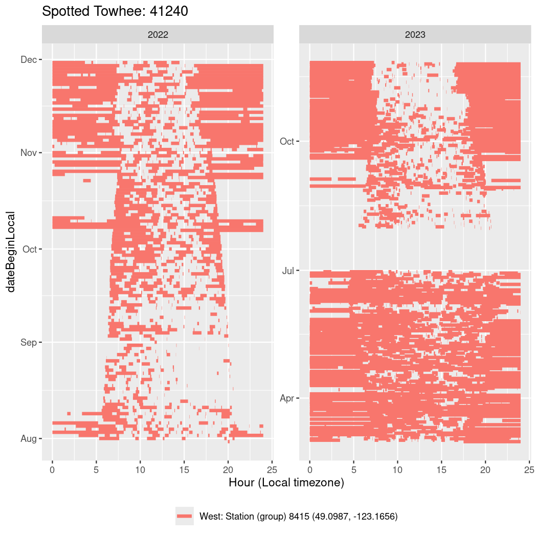
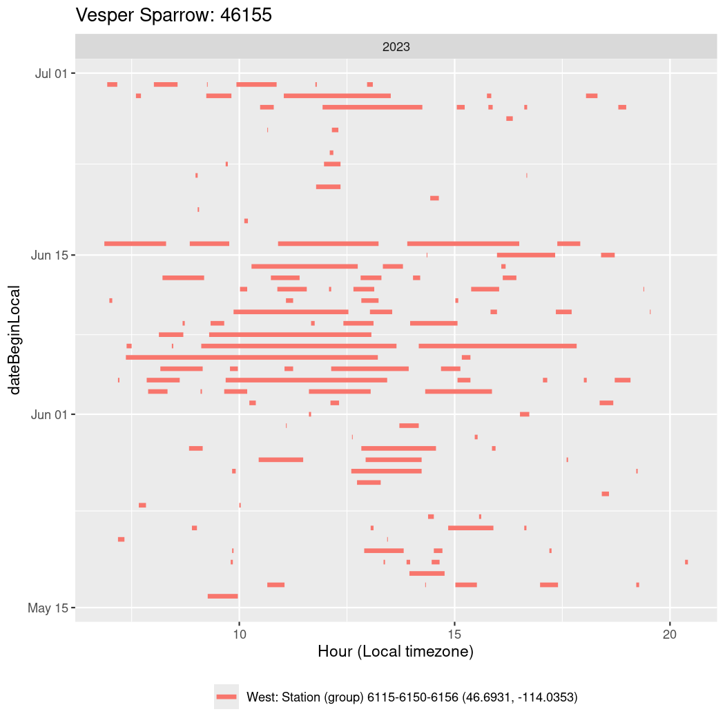
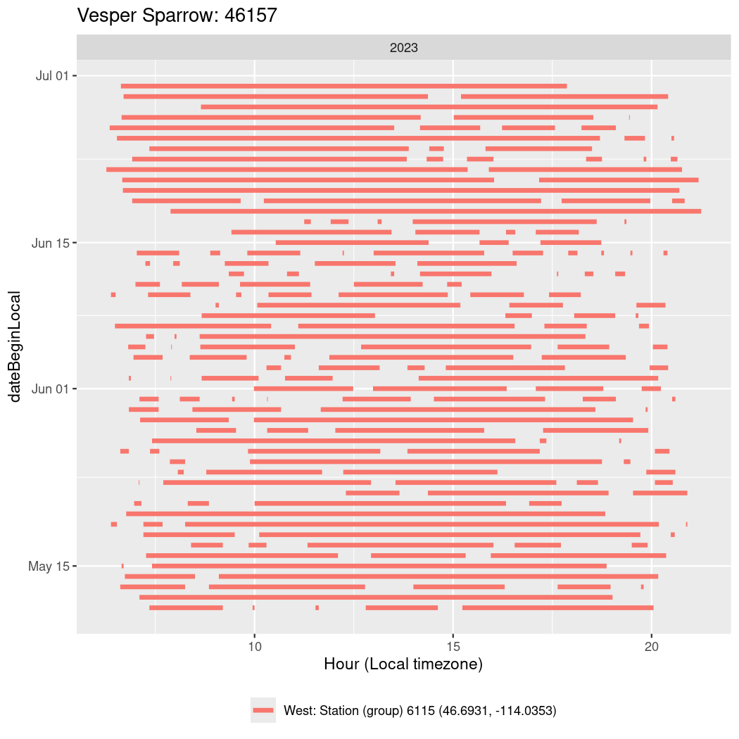
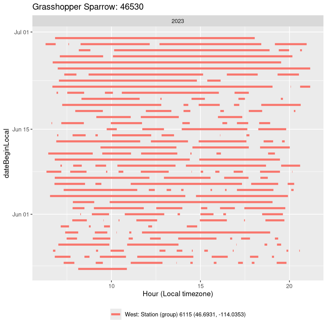
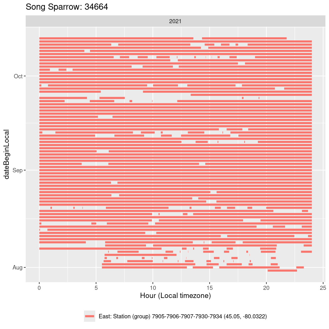
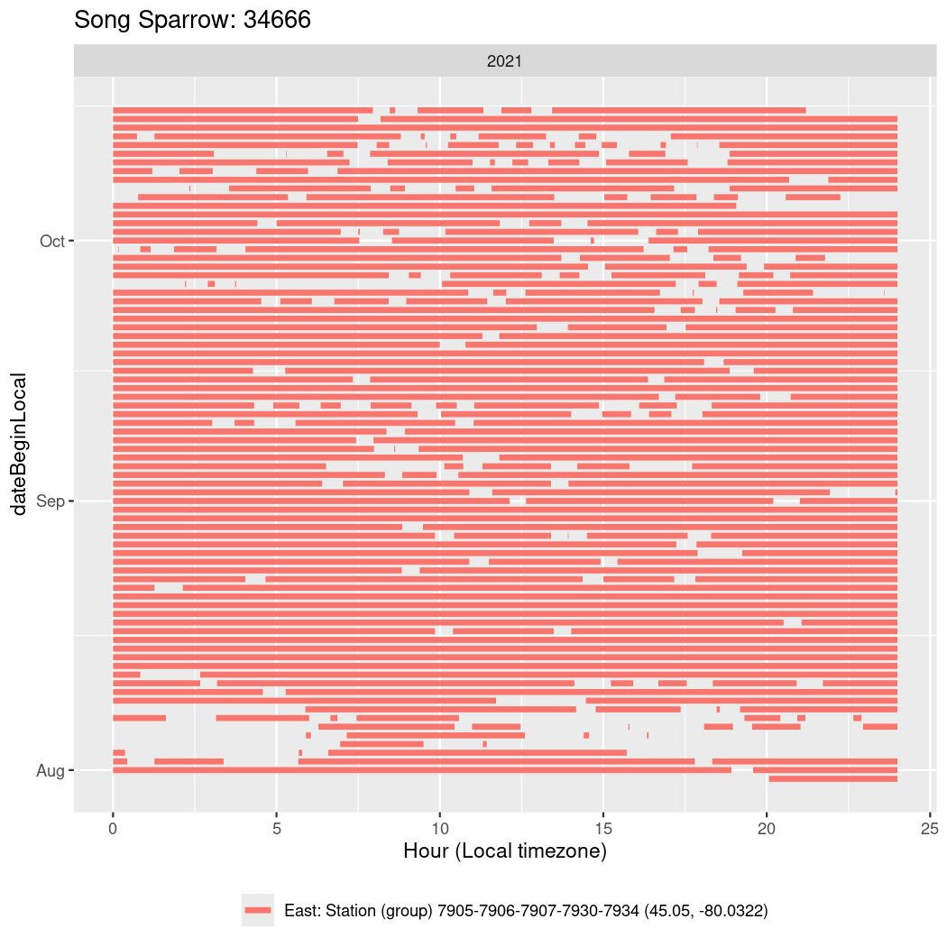
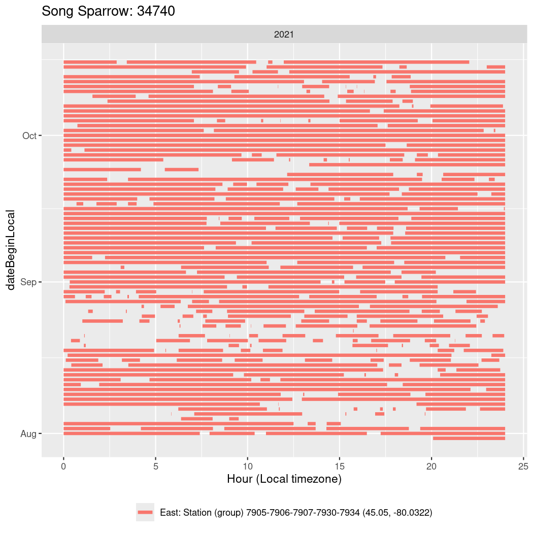
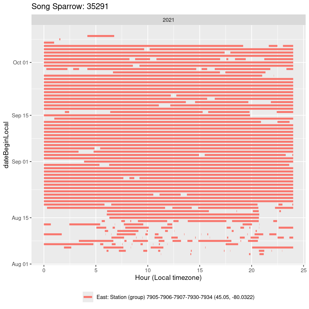
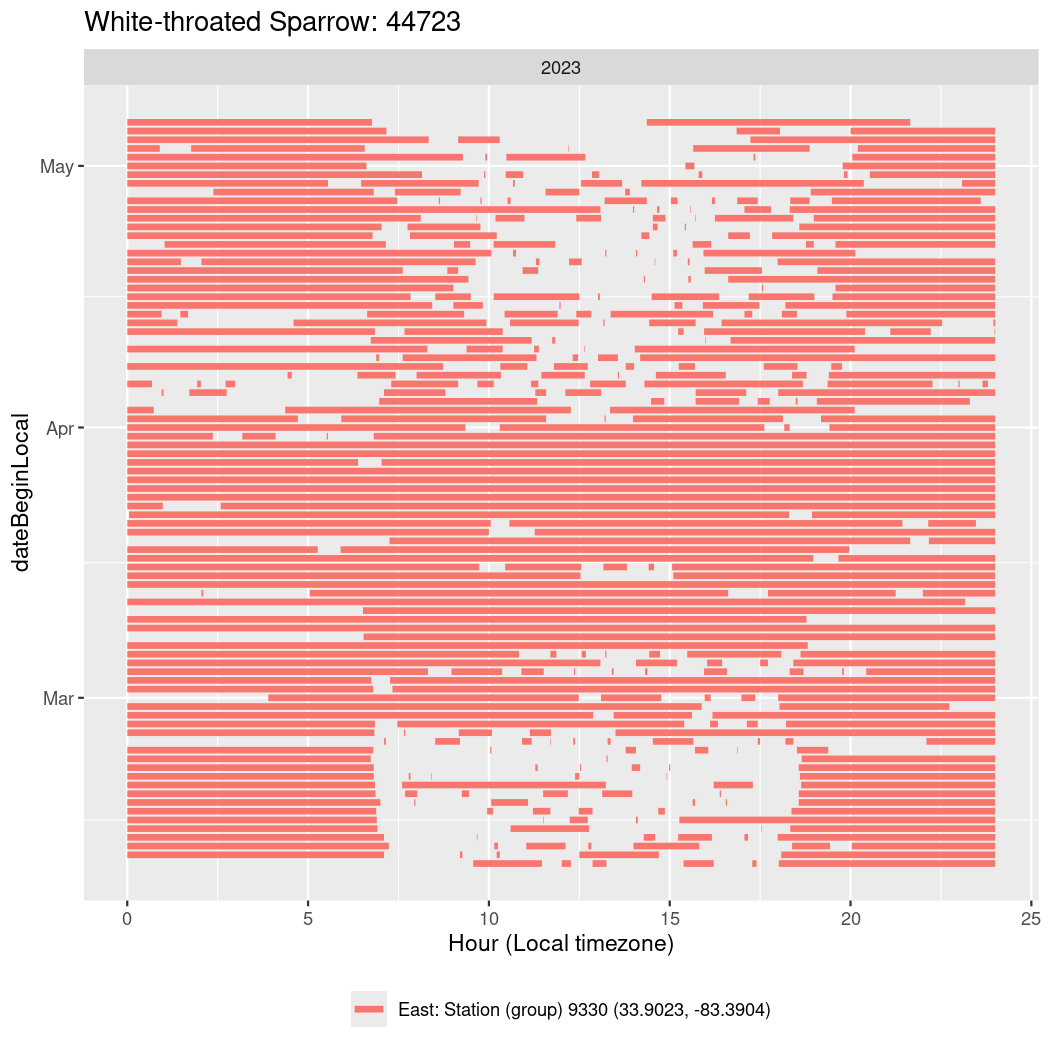
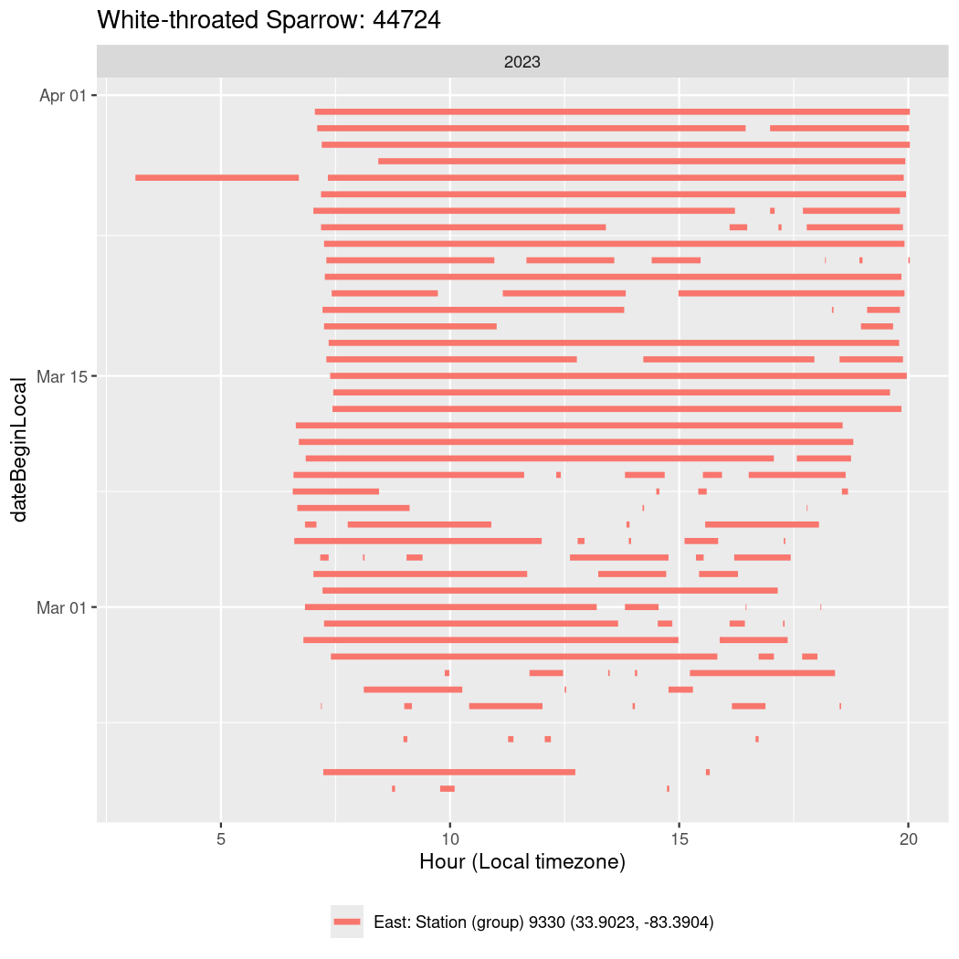
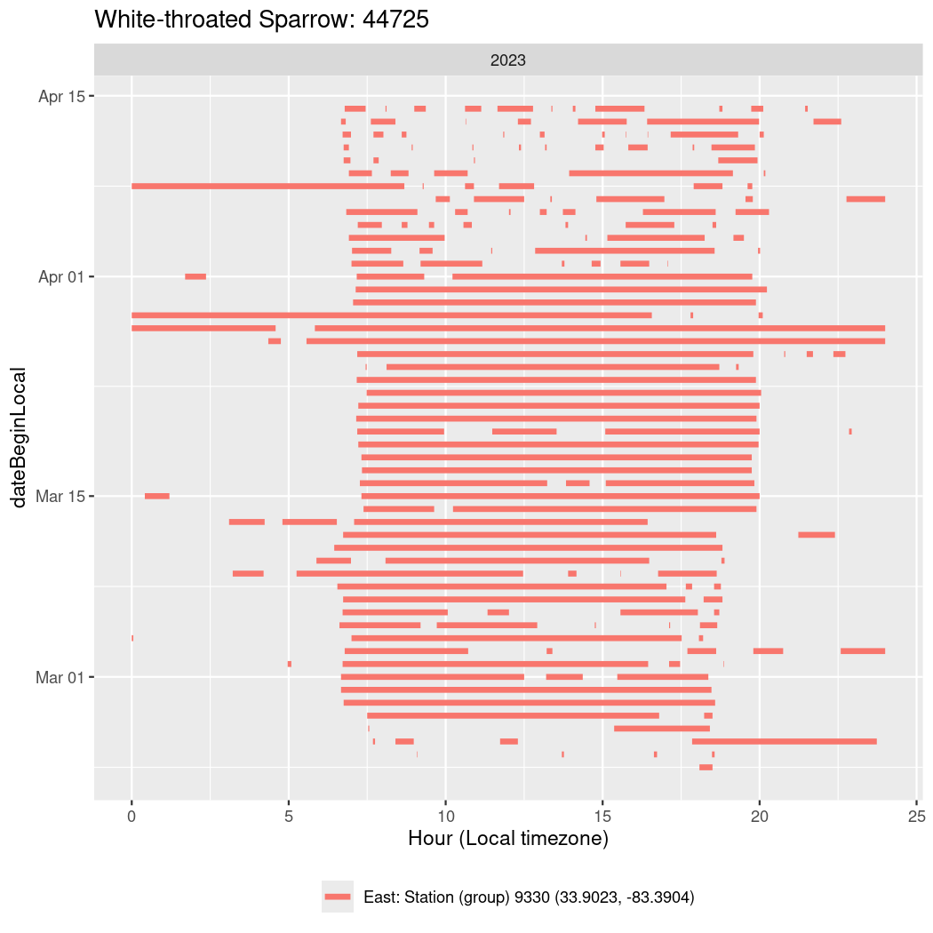
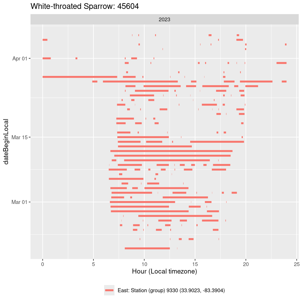
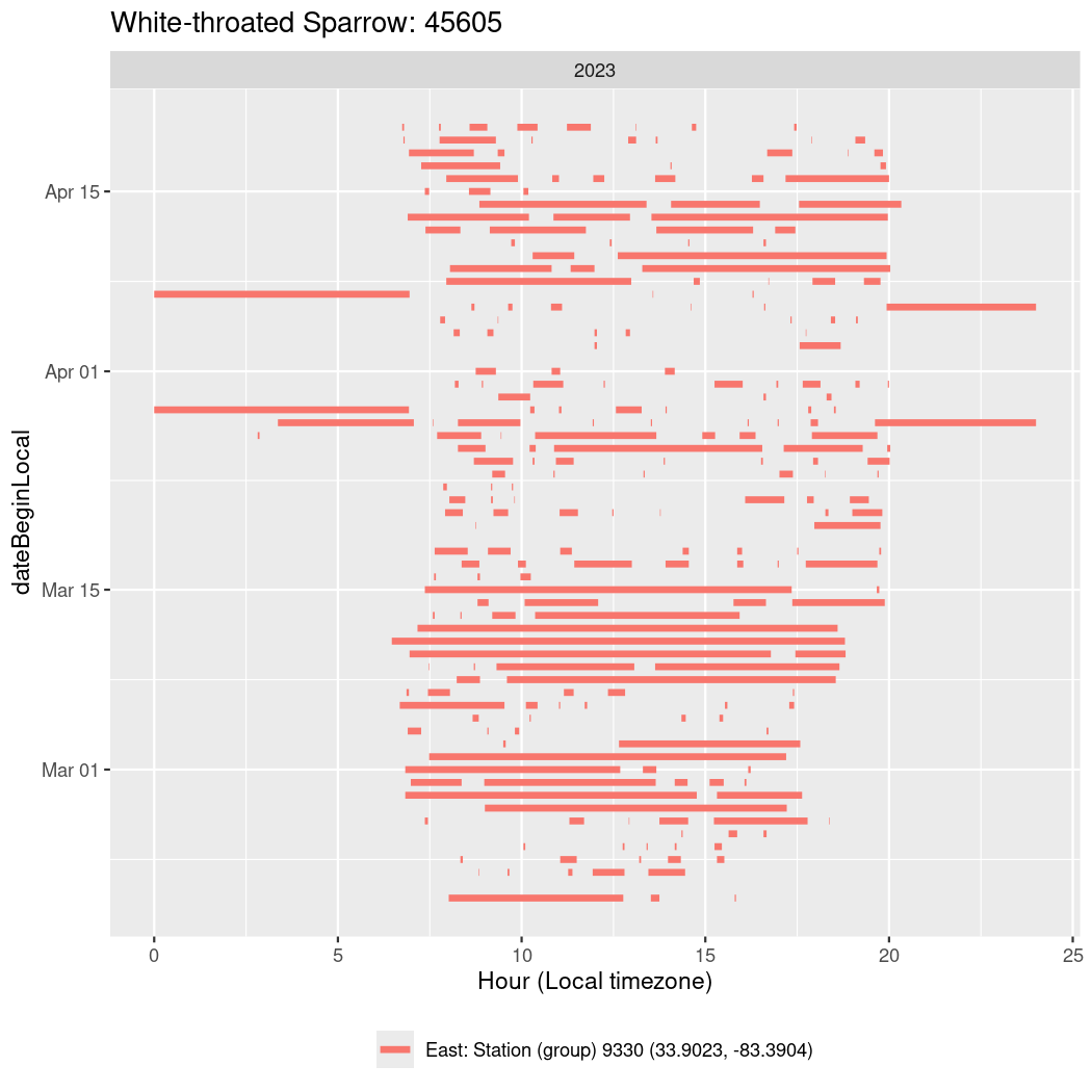
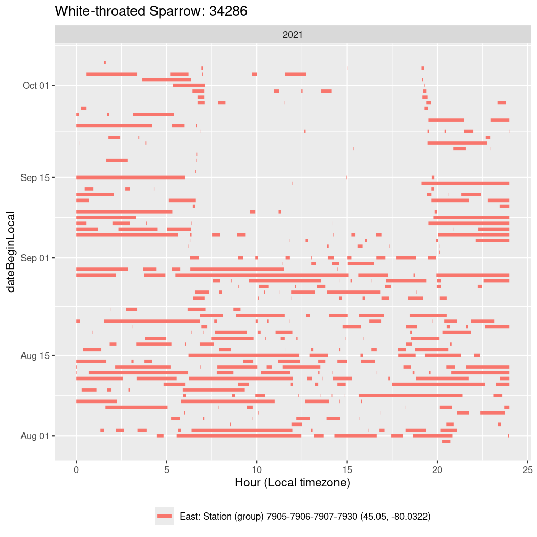
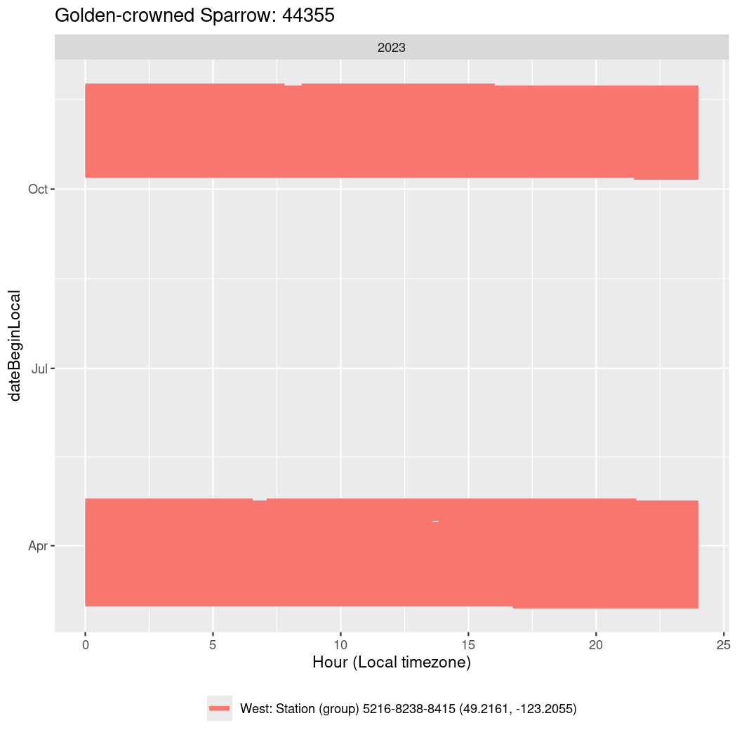
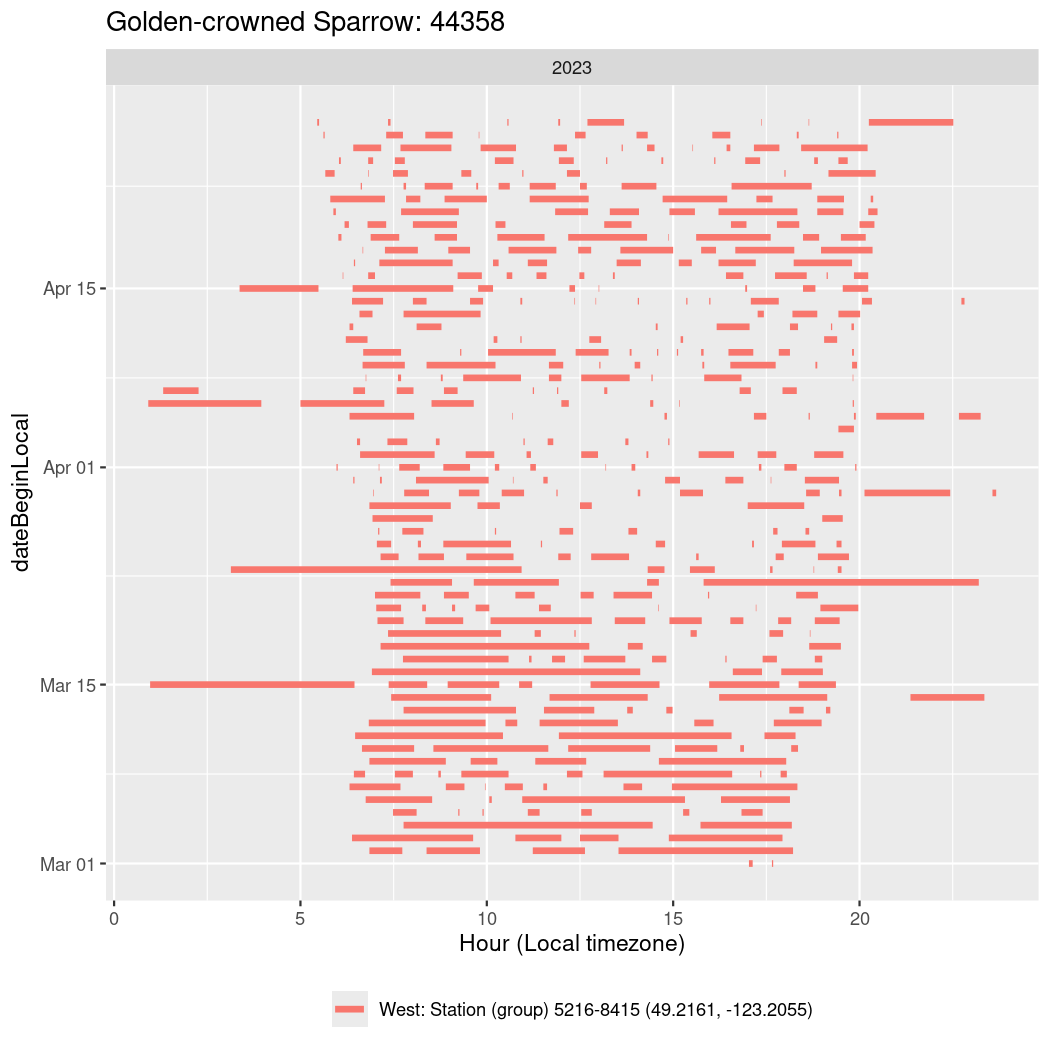
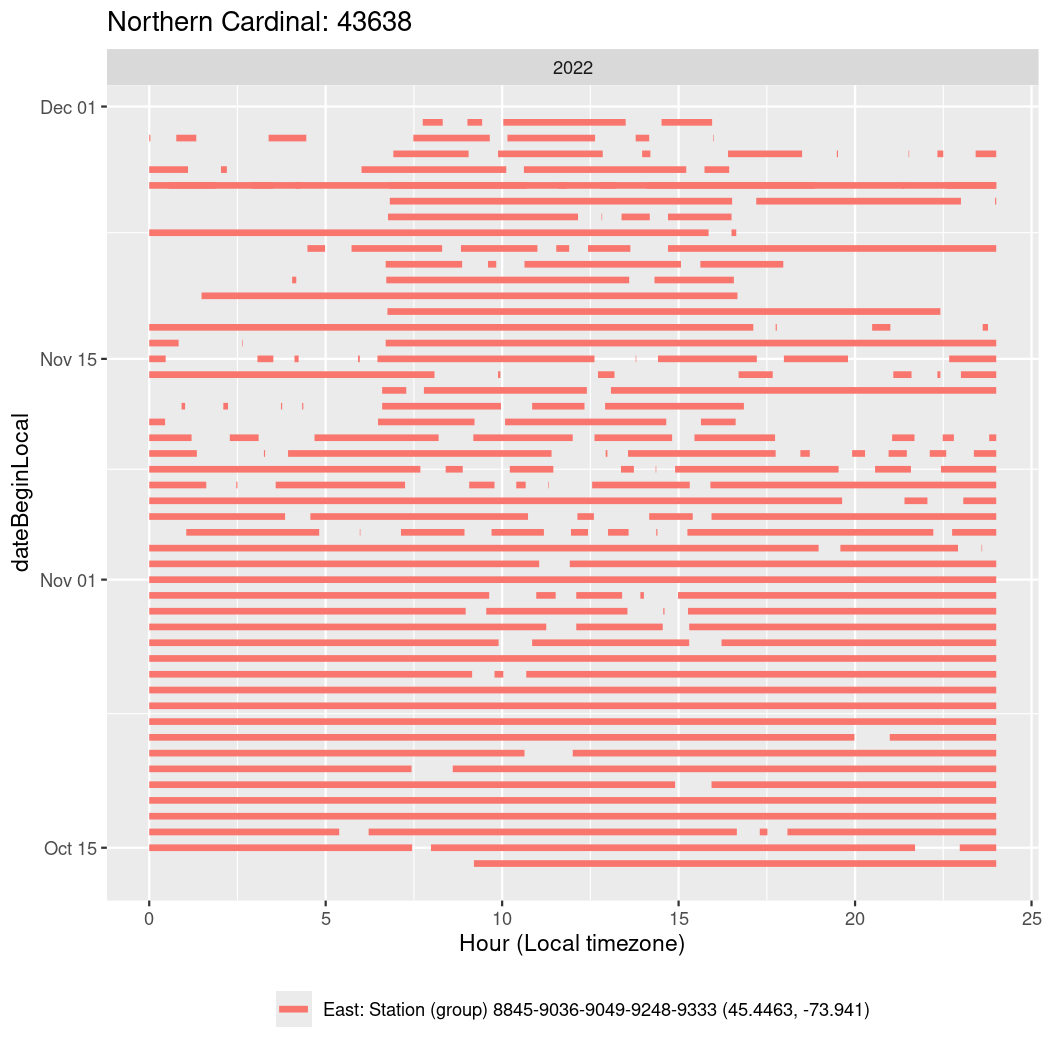
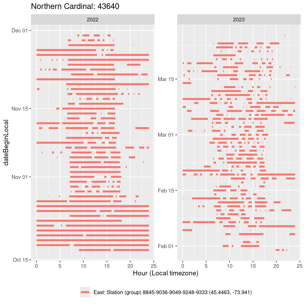
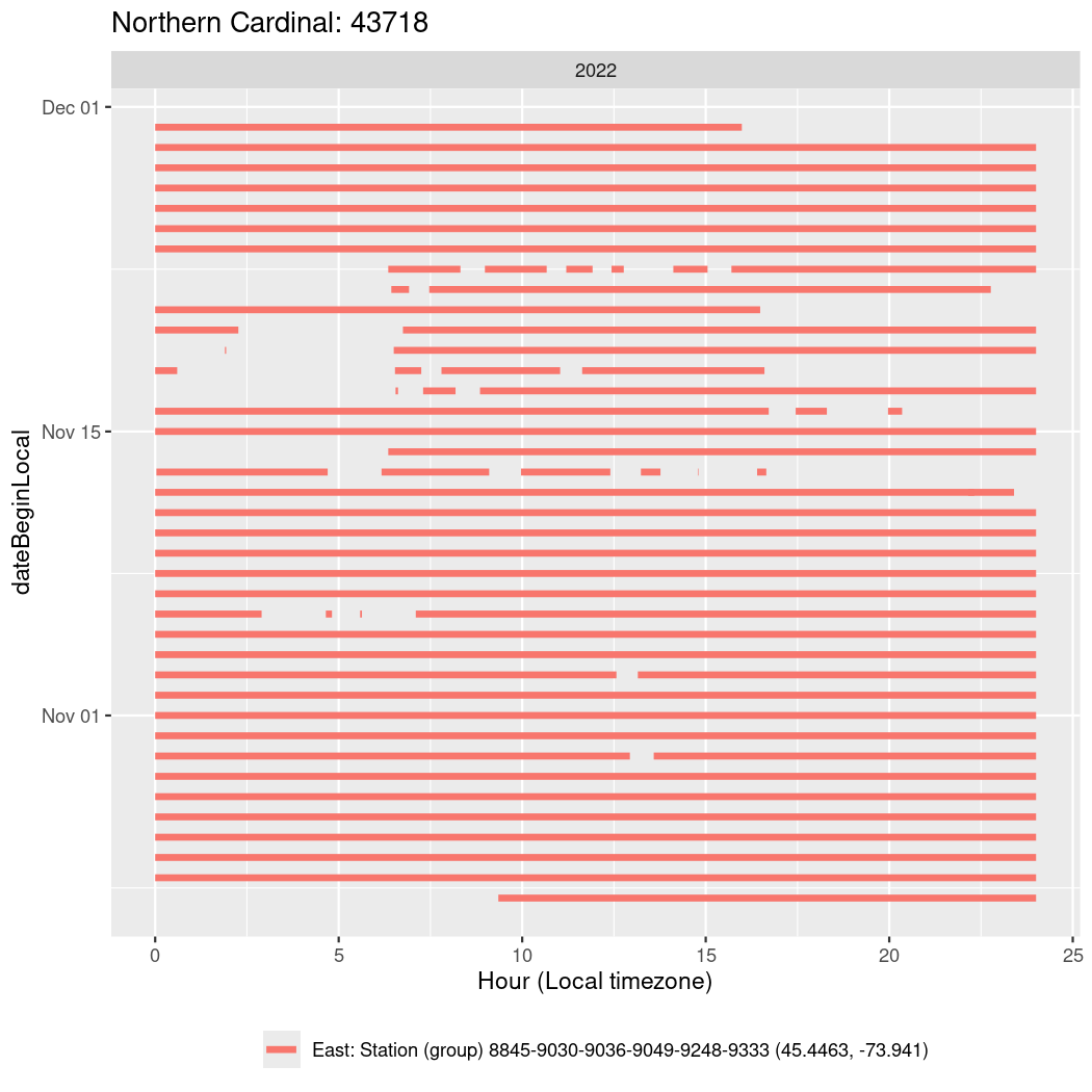
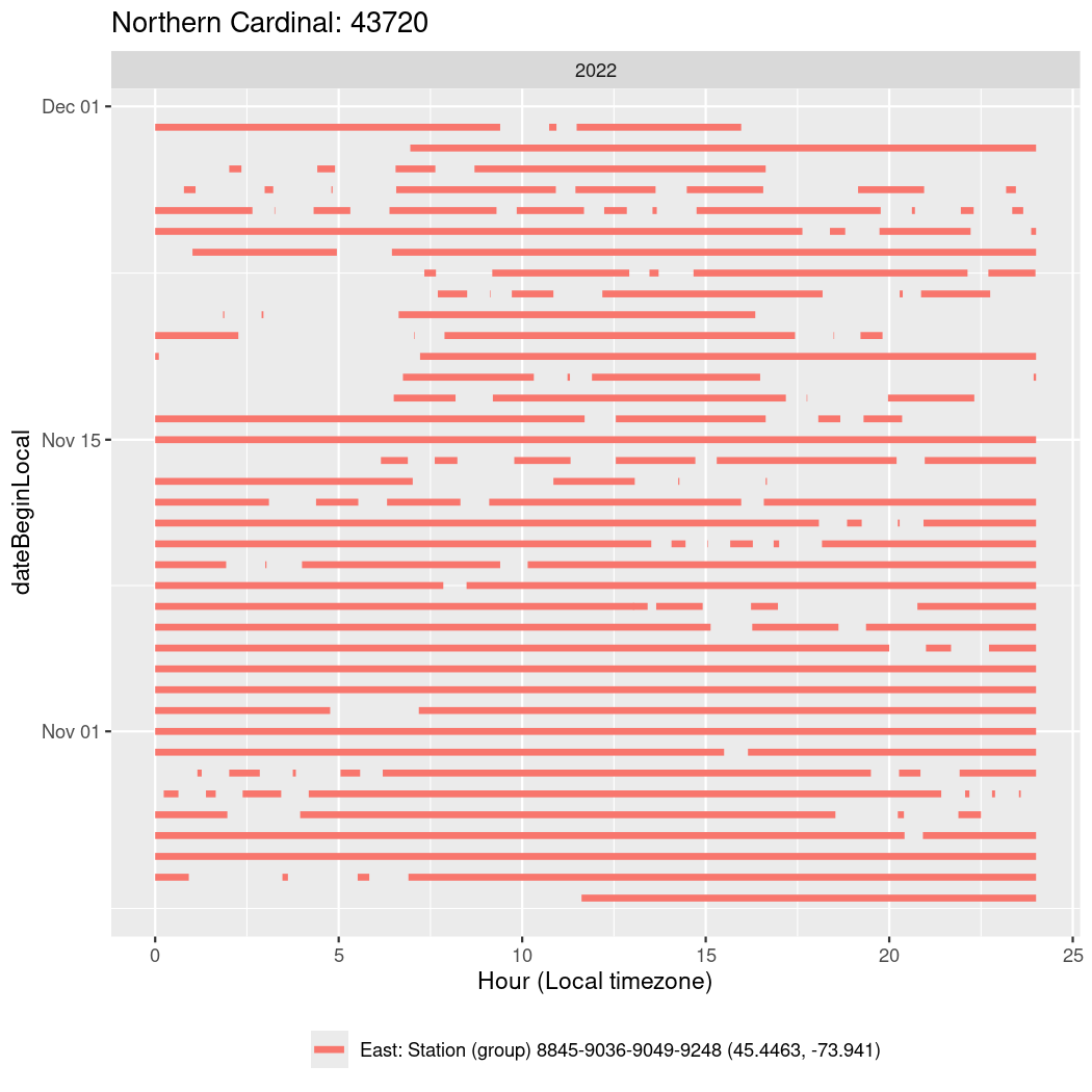
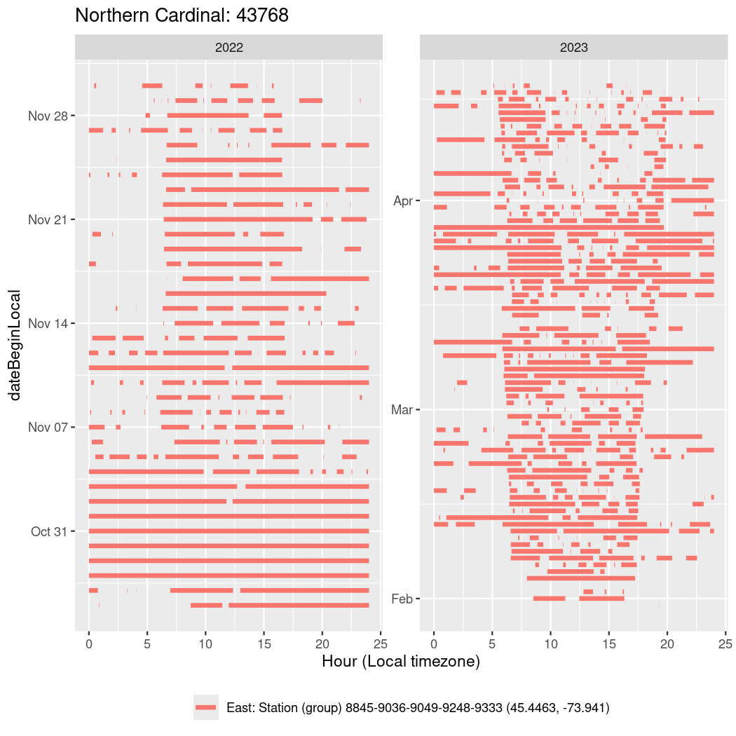
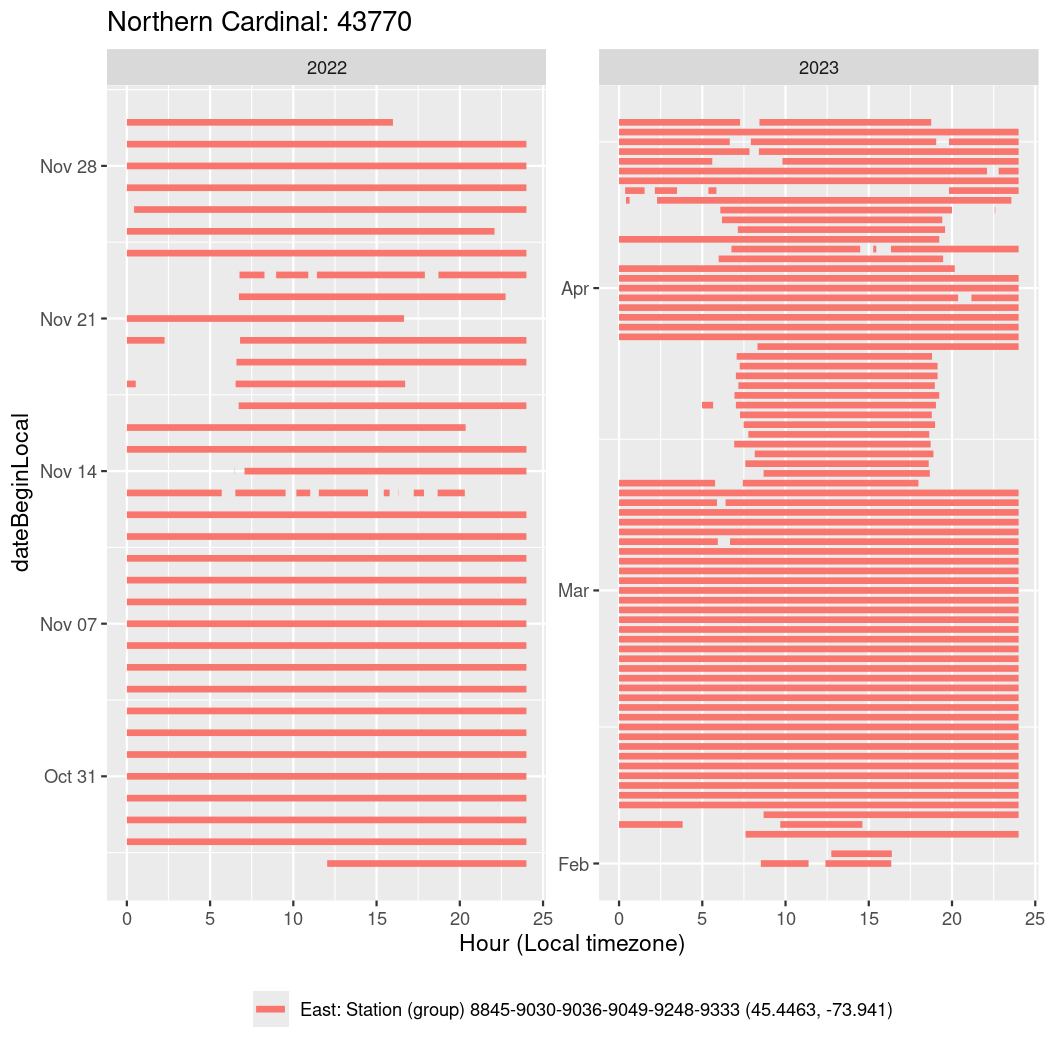
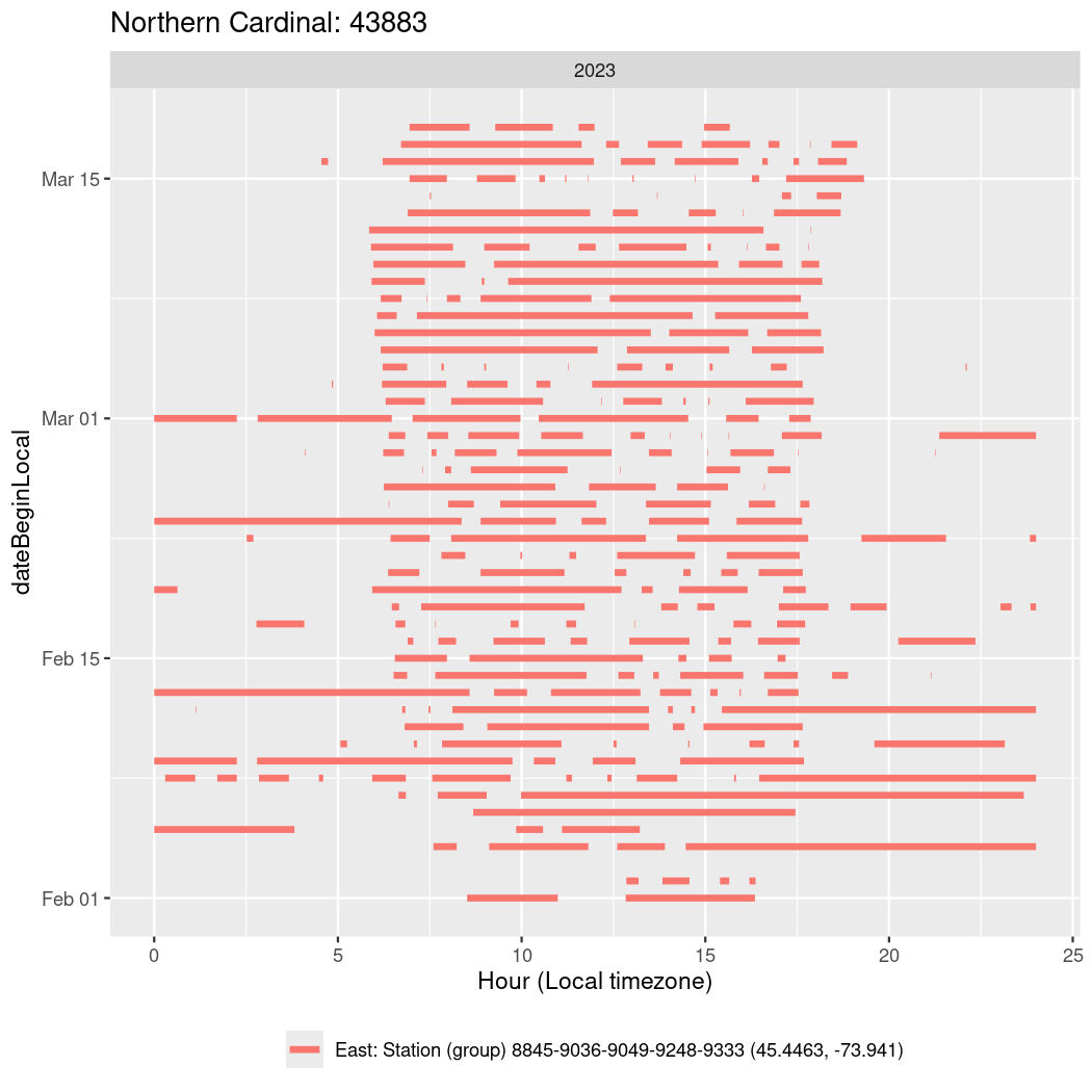
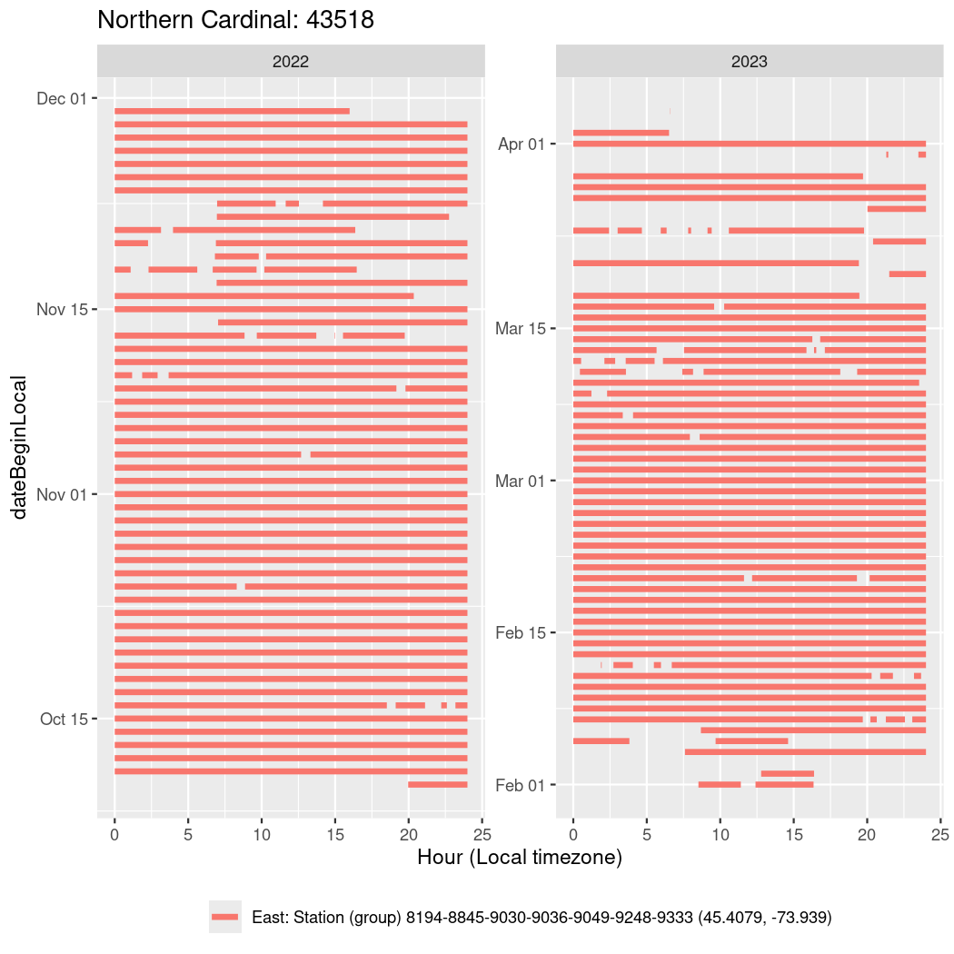
Now we’ll create circadian plots for each of these individuals for the dates at which they were consistently at a single station.
Code
walk(unique(circadian$tagDeployID), \(x) {
  cat("\n\n####", x, "\n\n")
  g <- ggplot(filter(circadian, tagDeployID == x),
         aes(x = start, xend = end, y = dateBeginLocal, colour = stn_nice)) +
    theme(legend.position = "bottom", legend.title = element_blank()) +
  geom_segment(linewidth = 1.5) +
  facet_wrap(~ year, scales = "free") +
  labs(title = paste0(circadian$english[circadian$tagDeployID == x], ": ", x),
       x = "Hour (Local timezone)")
  print(g)
})
48775
49778
41657
41673
35739
13846
18880
18897
17852
17853
17854
17855
18548
18876
18881
18886
18890
18894
18898
18899
18900
18901
18903

18904
18905
18910
18911
18912
18913
18914
19050
19410
19414
19417
43425
13844
13847

13859
14161
14163
14166
18885
35306
35309
35310
35473
35474
35475
35476
35477
35478
35480
35481
35485
35486
35740
35913
41579
41580
41676
41680
41700
42002
42241
42243
44752
49325
49570
49571
25846
40636
41197
17846
17850
18878
18879
18888
26766
13858
18547
18891
18892
35311
35482
35483
41539
39613
39601
39600
34276
34477
34277

34473
34475
34476
34478
34479
34480
34491
34668

34673
39119
39563
39584
39585
39612
39617
34272
34280
39592
34275
34489
34667
41215
41222
41246
45987
41206
41208
41209
41210
41211
41217
41218
41219
41220

41221
41224
41228
41229
41230
41231
41233
41239
41240
41248
45743
45744
45746
45750
45984
45985
47032
29524
29527
46155
46157
46759

47326
40492
41369
41372
41374
46156
46162
46164
46530
34665
34656
34657
34664
34666
34740
35291
35293
39121
39568
39574
39576
39586
39594
39610

39611
39626
34741
34281
39581
42487
42558
44485
44722
44723
44724
44725
45604
45605
34286
44355
44358
44359
44361
43460
43637
43638
43640
43718
43719

43720
43768
43770
43883
43518
43639
43979
51005
51154
51212
51404
47334
40491
40712
41367
41370
41373
46158
46159
46160
46161
46165
46532
46758
47322
47324
47328
47329
47333
47339
29521
29523
29525
35036
39572
39615
39548
39090
39550
Future Ideas
- Assess how many local station along the path were not used (but were active).
- Look at arrivals with respect to time of day to assess when birds arriving
- Use timing as indicator of passing through or stopping over? (i.e early morning?)
- Amie et al. use hit patterns and timing to determine if stopping in.
- Explore timing of activity during migration stop-overs
- Are birds leaving specific areas at particular times, then returning?
- see Looking at circadian patterns for a brief exploration